Enhancing PLL performance in weak grids: a comparative analysis of backward and bilinear ADC with SOGI-PLL

1. Introduction

Recently, research on water electrolysis systems has become active for Carbon Neutral. These systems receive voltage from the grid, creates DC voltage through an AC-DC converter, and creates voltage for the water electrolysis stack through a DC-DC converter. In AC-DC rectifier, Vienna rectifier is used for reasons high power factor and efficiency [1-3]. These systems are generally limited to installation locations near the sea. As a result, as the distance to the power grid from which the power is received increases, the electrical distance grows and the impedance of the system cannot be ignored. The large value of grid impedance negatively impacts the controller and PLL under weak grid conditions. Research on the grid impedance estimation [4-6], PLL methods and stability in weak grids [7-9].

On the other hand, the control system of a Vienna rectifier includes a PLL, DC-link voltage controller, input current controller, and PWM controllers based on DQ transformation. However, in weak grids, the PLL is affected by grid impedance. In addition, the switching distortion at Point of Common Coupling (PCC) voltage is affected by the DC-Link voltage included in the three-phase switching functions, and the voltage measurement at PCC affects the sampling. In this paper, a hardware LPF is applied to minimize the influence of switching functions during PCC voltage sensing. A SOGI-PLL structure is then introduced and proposes a conversion method by comparing the backward and bilinear methods according to the digital conversion method. In addition, the method to mitigate voltage drop issues caused by sampling delays is proposed and effectiveness is verified through PSIM simulation.

In this paper, Chapter 2 describes the configuration and control method of the Vienna rectifier. Chapter 3.1 explains the operating principle of SOGI PLL, Chapter 3.2 analyzes the digital conversion method and Chapter 3.3 explains the influence of switching distortion and hardware LPF. Chapter 4 explains simulation according to digital conversion method and hardware LPF and Chapter 5 contains the conclusion of the paper.

2. Vienna rectifier and control system

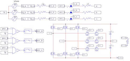
Fig. 1 is Vienna rectifier circuit in weak grid. It is a boost-based topology that receives grid AC voltage and increases the output voltage according to the duty. The voltage equation of the Vienna rectifier input voltage is a Eq. (1). The equation can be expressed in terms of the grid voltage ($e_a$), grid impedance voltage $\left(v_{L{g}_a}\right)$, filter impedance voltage$\left(v_{L{f}_a}\right)$, and terminal voltages AO $\left(v_{AO}\right)$ at both ends of the switch, and voltage $\left(v_{ON}\right)$ is the capacitor between the midpoint (O) and the neutral point (N). $e_b$ and $e_c$ can be obtained in the same way. From the voltage equation in Eq. (1), the expression for $v_{AO}$ and $v_{ON}$ can be derived, which are presented in Eq. (2) and (3) [10]. When Eq. (2) and (3) are substituted into Eq. (1), the resulting expression includes switching functions:

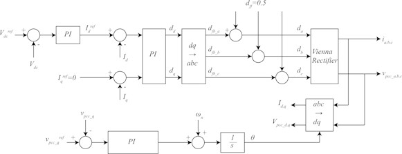
Fig. 2 shows the control block diagram of the Vienna rectifier. The PLL controller is used for measuring the PCC voltage. Create current reference through DC-Link voltage controller. Create duty reference through current controller.

Fig. 1Vienna rectifier circuit in weak grid

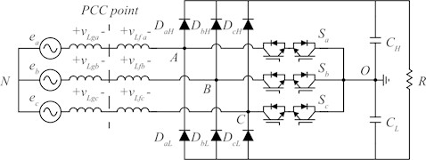
Fig. 2Control block diagram of the Vienna rectifier

3. SOGI-PLL fundamentals and robust digital realization under switching distortion

3.1. Operating principles of SOGI-PLL

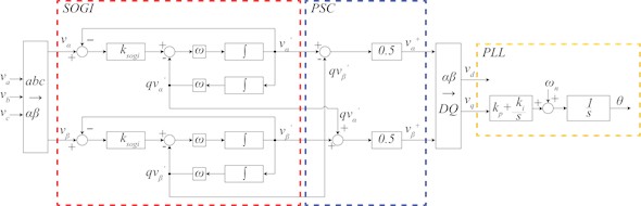
The SOGI-PLL transforms the input three-phase voltages into $\alpha \beta$ voltage components using the Clarke transformation. The $\alpha \beta$ voltages are processed through the SOGI to extract the Positive-Sequence Component (PSC), which are then converted into DQ voltages and used to obtain the phase angle $\theta$ through a Synchronous Reference Frame based PLL. The block diagram of SOGI-PLL is shown in Fig. 3, and each block is explained. The SOGI block generates $v_{\alpha }^{\text{'}}$, $q{v}_{\alpha }^{\text{'}}$, $v_{\beta }^{\text{'}}$ and ${qv}_{\beta }^{\text{'}}$ from the input $v_{\alpha }$ and $v_{\beta }$.

Fig. 3SOGI-PLL block diagram

The transfer function is arranged from the input $v_{\alpha \beta }$ and the output $v_{\alpha \beta }^{\text{'}}$, resulting in a Band-Pass Filter (BPF) shown in Eq. (4). This filter allows a specific frequency band to pass without causing phase delay. Similarly, when the transfer function is arranged from the input $v_{\alpha \beta }$ and the output ${qv}_{\beta }^{\text{'}}$, it results in a LPF, as shown in Eq. (5). This filter passes a frequency lower than a specific frequency and the phase is shifted by 90 degrees:

4

$D\left(s\right)=\frac{v_{\alpha ,\beta }^{\text{'}}}{v_{\alpha ,\beta }}=\frac{k_{sogi}{\omega }^{2}s}{s^2+k\omega s+{\omega }^2},$

5

$Q\left(s\right)=\frac{q{v}_{\alpha ,\beta }^{\text{'}}}{v_{\alpha ,\beta }}=\frac{k_{sogi}{\omega }^2}{s^2+k\omega s+{\omega }^2}.$

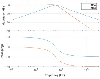
Fig. 4 is a graph of Eq. (4) and (5) in MATLAB of bode plot. In the bode plot, we can see that the $D\left(s\right)$ graph passes through a frequency of 60 Hz and there is no phase delay. $Q\left(s\right)$ passes frequencies lower than 60 Hz, but has a 90-degree phase delay.

Fig. 4D(s) and Q(s) bode plots of SOGI

The PSC block is explained in Fig. 3. Using their SOGI outputs the PSC $v_{\alpha \beta }^{+}$. The voltage vector can be organized as in Eq. (6) below. Eq. (7) is defined as follows:

6

$v_{abc}^{+}=\left[\begin{array}{ccc}{v}_a^{+}& v_b^{+}& v_c^{+}\end{array}\right],v_{abc}^{-}=\left[\begin{array}{ccc}{v}_a^{-}& v_b^{-}& v_c^{-}\end{array}\right],$

7

$T^{+}=\frac{1}{3}\left[\begin{array}{ccc}1& a& a^2\\ a^2& 1& a\\ a& a^2& 1\end{array}\right],T^{-}=\frac{1}{3}\left[\begin{array}{ccc}1& a^2& a\\ a& 1& a^2\\ a^2& a& 1\end{array}\right],a=e^{j\frac{2}{3}\pi },$

8

$v_{\alpha \beta }^{+}=\left[T_{\alpha \beta }\right]v_{abc},\left[T_{\alpha \beta }\right]=\frac{2}{3}\left[\begin{array}{ccc}1& -\frac{1}{2}& -\frac{1}{2}\\ 1& \frac{\sqrt{3}}{2}& -\frac{\sqrt{3}}{2}\end{array}\right],$

9

$v_{\alpha \beta }^{+}=T^{+}{v}_{abc}^{+}=\left[T_{\alpha \beta }\right]\left[T^{+}\right]v_{abc}=\left[T_{\alpha \beta }\right]\left[T^{+}\right]{\left[T_{\alpha \beta }\right]}^T{v}_{abc}=\frac{1}{2}\left[\begin{array}{cc}1& -q\\ q& 1\end{array}\right]\left[\begin{array}{c}{v}_{\alpha }\\ v_{\beta }\end{array}\right].$

Eq. (8) can be obtained using Clarke transform. For PSC $\alpha \beta$ voltage, it can be obtained through each $\alpha \beta$ combination. The organized equation is shown in Eq. (9). To extract the 60 Hz component of the grid voltage from the PSC, the SOGI-PLL is designed to have corner frequency at 60 Hz. The PSC voltage $v_{\alpha \beta }^{+}$, obtained from Eq. (9), is transformed into the DQ domain using the Park transformation. The $Q$-axis voltage component derived from this transformation is used for the PLL operation. After PI control, the fundamental frequency compensation $\left({\omega }_n\right)$ is added and integrated to estimate $\theta$. It is used to apply DQ transformation.

3.3. Improved PSC under switching distortion using LPF-assisted SOGI-PLL

When Eq. (1) and Eq. (3) are expressed in terms of the PCC voltage, it can be represented as shown in Eq. (12). It shows that in PCC voltage of the weak gird, the voltage can be combined with the grid voltage ($e_a$) and the grid impedance voltage ($v_{L{g}_a}$) as $v_{Pc{c}_a}$. Additionally, the PCC voltage is expressed of the filter impedance voltage ($v_{Lf}$) and the three-phase switch function as a DC voltage multiplication. When measuring PCC voltage, it is difficult to measure PSC of PCC voltage even if sampling at the same or twice the switching frequency. This problem causes switching distortion problems. To mitigate the influence of switching distortion, an LPF is implemented in hardware. By applying the hardware LPF, the switching distortion in the measure PCC voltage is significantly reduced, enabling more accurate voltage detection:

12

$v_{pc{c}_a}=v_{L{f}_a}+v_{AO}-\frac{1}{3}\left(v_{AO}+v_{BO}+v_{CO}\right).$

Fig. 6 shows the PSIM diagram when hardware LPF is applied. As shown in Fig. 6, a hardware LPF is applied to reduce the switching distortion when measuring the PCC voltage. Therefore, after the switching distortion is reduced through the LPF, the PCC voltage is measured.

Fig. 5BPF and LPF bode plots according to digital conversion method

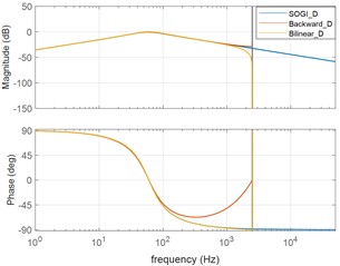
a) Bode plot of BPF

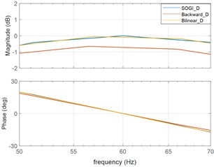
b) Magnified view around 60 Hz of BPF

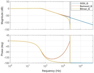
c) Bode plot of LPF

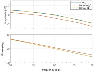
d) Magnified view around 60 Hz of LPF

Fig. 6PSIM diagram with hardware LPF

4. Simulations

The PSC was extracted using SOGI-PLL following the application of a hardware LPF, and the proposed digital conversion method was verified through PSIM simulation. Table 1 summarizes the simulation parameters.

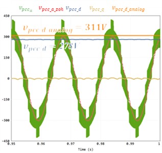
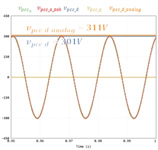
Fig. 7(a) shows the voltage waveform using the backward method. The second waveform is the $\alpha$ axis voltage through SOGI. Each is an analog voltage and a voltage in backward method. The analog voltage peak is 311 V, and the voltage in the backward method is 288 V. The difference between the two is 23 V. This has a 6.7 % error between the backward method voltage and analog voltages. It can be confirmed that an error occurs in the D-axis as well by performing DQ transformation through PSC. Fig. 7(b) presents the result using the bilinear method. The second waveform is the $\alpha$ axis voltage through SOGI. Each is an analog voltage and a voltage in bilinear method. The analog voltage is 311V, and the voltage in the backward method is 311 V. In this case, there was almost no error between the bilinear method voltage and analog voltages, and the D-axis voltage also showed accurate tracking. Fig. 7(c) the waveform in a weak grid without hardware LPF applied. Orange color and blue color are the PCC voltages for DQ transformation. Orange color is the analog voltage of 311 V and blue is the PCC D-axis voltage without hardware LPF of 278 V. Due to switching distortion, the PSC voltage includes distortion, resulting in voltage error. On the other hand, Fig. 7(d) shows the waveform when the hardware LPF is applied. Orange color and blue color are the PCC voltages for DQ transformation. Orange color is the analog voltage of 311 V and blue color is the PCC D-axis voltage with hardware LPF of 301 V. The difference between the two is 10 V. In this case, the effect of switching is minimized, allowing accurate PSC extraction and small error voltage measurement.

Fig. 7Voltage waveform according to digital conversion method and hardware LPF application

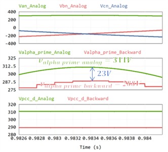
a) Waveform with backward method

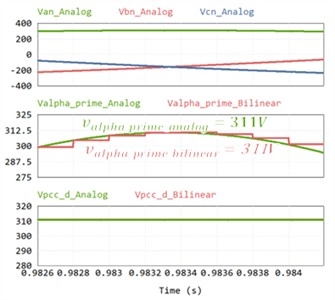
b) Waveform with bilinear method

c) Waveform without hardware LPF

d) Waveform with hardware LPF

5. Conclusions

In this paper, a digital conversion method for the SOGI-PLL and the application of a hardware LPF are proposed to ensure stable PLL operation under weak grid conditions. It was analyzed according to the digital conversion method. The backward method has an error of 7.4 % compared to the analog voltage. On the other hand, the error of the bilinear method is close to 0 and it was confirmed that there is an improvement effect of 7.4 %. The bilinear method is proposed for digital conversion. To reduce switch distortion for stable SOGI-PLL operation, hardware LPF was used. When hardware LPF was not used, the error of $v_{pc{c}_d}$ was confirmed to be about 10 % of $v_{pc{c}_d}$ occurred. However, when hardware LPF was used, it was confirmed that the error was reduced to 2.5 %. The error was reduced by 7.5 %, from 10 % to 2.5 %. This paper analyzed the performance of SOGI-PLL according to its digital conversion method and confirmed the impact of hardware LPF. In addition, the use of a hardware LPF and SOGI-PLL was proposed to enhance the operational stability of the PLL under weak grid conditions.