Field characterization of urban road traffic noise sources: effects of road class and vehicle composition

2.1. Field monitoring campaign

Field monitoring was undertaken on selected sections of 25 urban roads in Guangzhou, China, as shown in Table 1. The sample covered four road classes – expressway, arterial, secondary and branch road – and measurement positions were located between intersections, more than 50 m from the nearest one, and kept fixed for all visits.

At each section and operating period, three repeated measurements of 20 min were made. Levels and audio recordings were acquired with a Class 1 precision integrating sound level meter conforming to IEC 61672-1:2013 [19]; the microphone faced the carriageway at 0.2 m from its edge and 1.4 m above ground, following the roadside arrangement required by HJ 640-2012 [20]. A Class 1 acoustic calibrator conforming to IEC 60942:2017 [21] was applied at its 1 kHz, 94 dB reference setting before and after every session, and the result recorded. Field procedures followed the Chinese routine monitoring specification [20] and ISO 1996-2:2017 [22].

Traffic was counted continuously during each acoustic record, and vehicles were classified as small, medium or heavy following the Chinese road traffic noise assessment method [10]; average speed was estimated where a stable value could be obtained.

The operating periods were daytime off-peak (14:30-16:30), daytime peak (17:30-19:00) and night-time (22:00-24:00), the latter consistent with the definition of night in Chinese legislation [23]. Each section-period therefore yields one source-side level, obtained by averaging the repeated records, and one set of traffic values, as summarized in Table 1.

2.2. Acoustic and traffic indicators

The primary response variable was the equivalent continuous A-weighted sound level, $L_{Aeq,T}$, calculated from a discrete record of A-weighted levels as:

where $N$ is the number of discrete A-weighted samples in the 20 min record and $L_{A,k}$ is the $k$th A-weighted level. Traffic intensity for class $i$ was expressed as a flow rate $q_i=N_i/T$, where $N_i$ is the number of vehicles of class $i$ counted during $T=$ 20 min; flows are therefore reported per 20 min record and speeds in km/h. Associations between $L_{Aeq}$ and the traffic variables were described with the Pearson correlation coefficient:

where $n$ is the number of paired observations, $x_i$ and $y_i$ are the paired values of the two variables, and the barred symbols denote the sample means. The coefficient is used only as a descriptive measure of association, and no causal relation is implied. Within-section contrasts are expressed as $dL=L_{Aeq,2}-L_{Aeq,1}$, a positive value denoting a higher level under condition 2.

2.3. Metrological and statistical treatment

Class 1 instrumentation was used because the applicable standard requires a meter of class 1 or better [11]. The maximum permitted expanded uncertainty of a Class 1 sound level meter at reference conditions is 0.7 dB [19] and the permitted deviation of a Class 1 acoustic calibrator is 0.3 dB [21]; as the dominant Type B contributions these give an expanded uncertainty of about 0.8 dB for a single reported level [24]. Differences smaller than this are not interpreted, although part of the systematic contribution cancels when two levels from the same instrument are subtracted.

The three repeated records of a section-period were averaged, after rejection of outliers, to a single source-side level, so repeated records were not treated as independent observations and pseudo-replication was avoided; the statistics below therefore refer to $N=$ 75 section-period observations. Minimum-maximum intervals describe the observed spread of the sampled sections and are not confidence intervals. Correlations were tested two-tailed and are reported with 95 % confidence intervals obtained by Fisher z-transformation; because eight traffic variables were examined, a Bonferroni-adjusted threshold (alpha = 0.00625) is also indicated.

3.1. Source strength across road classes and periods

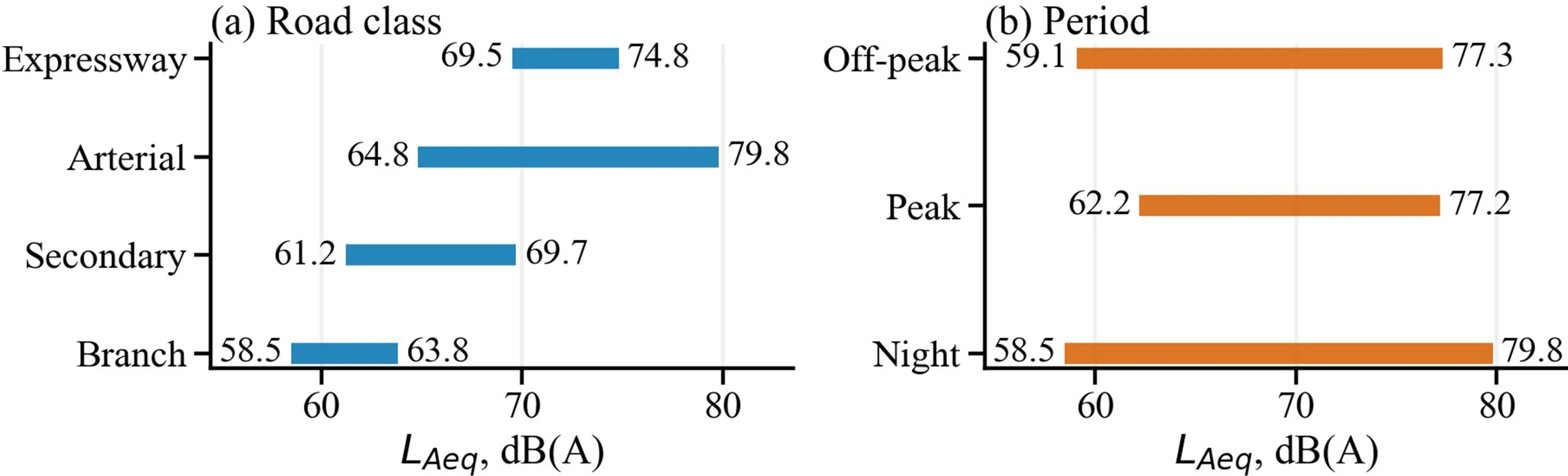
Levels across the 25 sections ranged from 58.5 to 79.8 dB(A), and their intervals differed by road class (Fig. 1(a)): expressways 69.5-74.8 dB(A), arterial roads 64.8-79.8 dB(A), secondary roads 61.2-69.7 dB(A) and branch roads 58.5-63.8 dB(A). The arterial interval (15.0 dB(A)) is an order of magnitude wider than the expanded uncertainty of a reported level (about 0.8 dB(A)), so the spread between sections is real rather than measurement scatter; intervals are observed ranges of the sampled sections, not confidence intervals.

The three periods overlapped substantially (Fig. 1(b)): 59.1-77.3 dB(A) in daytime off-peak, 62.2-77.2 dB(A) in daytime peak and 58.5-79.8 dB(A) at night. The greatest difference between periods at one section was 5.3 dB(A), and no uniform ranking by period was found: both increases and decreases occurred at individual sections, as the within-section comparisons below show.

Fig. 1Observed source-side LAeq intervals by a) road class and b) monitoring period

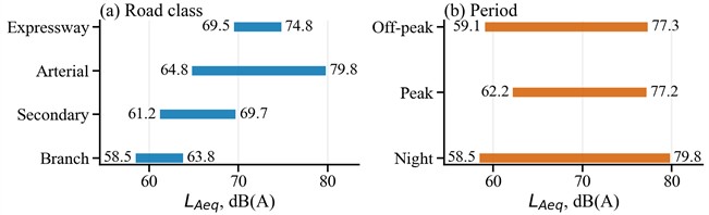
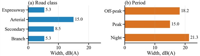
Fig. 2 separates level position from interval width: the width ranged from 5.3 dB(A) for expressways and branch roads to 15.0 dB(A) for arterial roads, and from 15.0 dB(A) at daytime peak to 21.3 dB(A) at night.

Fig. 2Observed minimum-maximum widths of the source-side LAeq intervals

3.2. Associations with traffic volume and vehicle composition

Flows correlated more strongly with the source-side level than the corresponding average speeds (Fig. 3). Correlations with total, small-, medium- and heavy-vehicle flow were $r=$ 0.794 (95 % CI 0.692-0.865), 0.782 (0.675-0.857), 0.867 (0.797-0.914) and 0.694 (0.554-0.796), all significant at p < 0.001 before and after Bonferroni adjustment. Speed correlations were weaker: 0.335 ($p=$ 0.003), 0.306 ($p=$ 0.008), 0.455 ($p<$ 0.001) and 0.186 ($p=$ 0.110); after Bonferroni adjustment only the correlations with total-vehicle and medium-vehicle speed remained significant.

Fig. 3Correlations between the source-side LAeq and traffic-flow or average-speed variables. Whiskers are 95 % confidence intervals (N= 75)

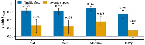
Medium-vehicle flow showed the strongest association and heavy-vehicle flow the weakest, but the confidence intervals of the medium-vehicle and total-flow coefficients overlap, so the two are treated as equivalent descriptors rather than as a ranking. Average speed varied over a much narrower range than flow, which may limit its descriptive value.

3.3. Illustrative operating-condition contrasts

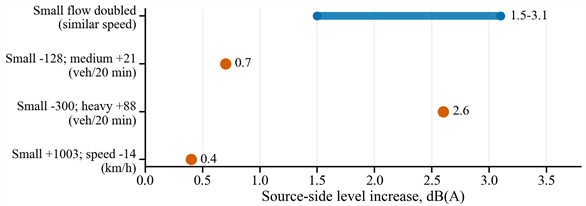
Four within-section comparisons examined whether these associations also appear at individual sections (Fig. 4). Where medium- and heavy-vehicle shares were similar at an arterial section, a doubling of small-vehicle flow accompanied a 1.5-3.1 dB(A) increase. At the same section the transition to night-time removed 128 small vehicles per 20 min but added 21 medium vehicles, and the level rose by 0.7 dB(A), which is comparable with the expanded measurement uncertainty and therefore treated as marginal. At an expressway section 88 additional heavy and 18 additional medium vehicles accompanied a 2.6 dB(A) increase, the largest of the four comparisons. At a secondary road section 1003 additional small vehicles with a 14 km/h speed reduction changed the level by only 0.4 dB(A), which is also within measurement uncertainty.

These are illustrative site-specific examples rather than per-vehicle estimates; they indicate that total flow alone may not describe source-side level changes when composition or speed differs.

Fig. 4Observed source-side level changes in the selected traffic contrasts

4.1. Novelty relative to established assessment and control practice

Mapping and prediction remain the appropriate tools for assessing exposure over large areas, and the present field data address a different question. A mapping calculation starts from an assumed traffic state, applies emission coefficients and propagation terms and returns a level at a receiver, so its result depends on how well that assumed state represents reality. The measurements quantify part of the variation hidden inside that assumption: one road class spanned 15.0 dB(A) and one operating period 21.3 dB(A). Table 2 compares this description with the frameworks and control practices used in different countries.

For control, the cause of an elevated level must be identified before a measure is selected. Barriers, quiet pavements, speed management and traffic restraint act on different parts of the source-path system [16-18]: a barrier or a quiet pavement cannot compensate for an increase produced by a larger share of heavy vehicles, and volume-based management cannot compensate for a composition effect. The results indicate that fleet composition most often distinguished one section-period from another: medium-vehicle flow was the strongest correlate and the largest within-section increase occurred where heavy-vehicle flow rose at night while total flow fell. The novelty here lies in that combination - a multi-city evidence base, an explicit uncertainty statement and a monitoring recommendation - rather than in a new prediction formula.

4.2. Implications for monitoring practice

The results support a modest extension of routine practice: records should retain vehicle counts disaggregated by class rather than a total volume, so that a measured level can be attributed to traffic volume, fleet composition or both. This requires no additional instrumentation and determines which mitigation measure is appropriate.

The uncertainty statement of Section 2.3 should accompany the measurement, so that differences below about 0.8 dB(A) are not reported as findings; the intervals and within-section differences measured here give realistic bounds for a survey of this size. Road class remains useful for stratification but is insufficient for explaining a specific measured level.

4.3. Limitations

The study is limited to 20 min records at selected Guangzhou sections and to descriptive statistics; it did not estimate causal emission coefficients, model propagation or residential exposure, and road-surface type, gradient, meteorology and driver behavior were not resolved. A transferable source model would require synchronized vehicle trajectories, other seasons and more road classes.