Abstract
A compact coupled model is developed for a low-frequency cavitator with two oppositely moving perforated grates. Mechanical oscillations are linked to voltage-driven coil dynamics, variable air gaps, magnetic saturation, nonlinear hydraulic resistance, liquid added mass, and finite-rate vapor-fraction evolution. Simulations for water at 80°C and an absolute chamber pressure of 0.38 MPa cover 41-100 Hz. For the adopted parameter set, the model predicts that the pressure threshold is crossed over approximately 41-60 Hz. At 50 Hz, the predicted grate amplitude is 2.21 mm, the minimum local pressure is 41.2 kPa, the peak vapor fraction is 4.8 %, and the RMS coil current is 2.81 A. The predicted total electrical input to the two drives is approximately 0.65 kW, while the fundamental dissipative component of the hydrodynamic load corresponds to an equivalent damping of about 138 N·s/m. The calculated phase lags demonstrate that prescribed in-phase harmonic mechanical forcing is inadequate. The model supports preliminary operating-point selection, while its magnetic and hydraulic coefficients require experimental identification. Published experiments on related devices provide technological context; direct validation of the present model and its extension to other fluid rheologies remain future work.
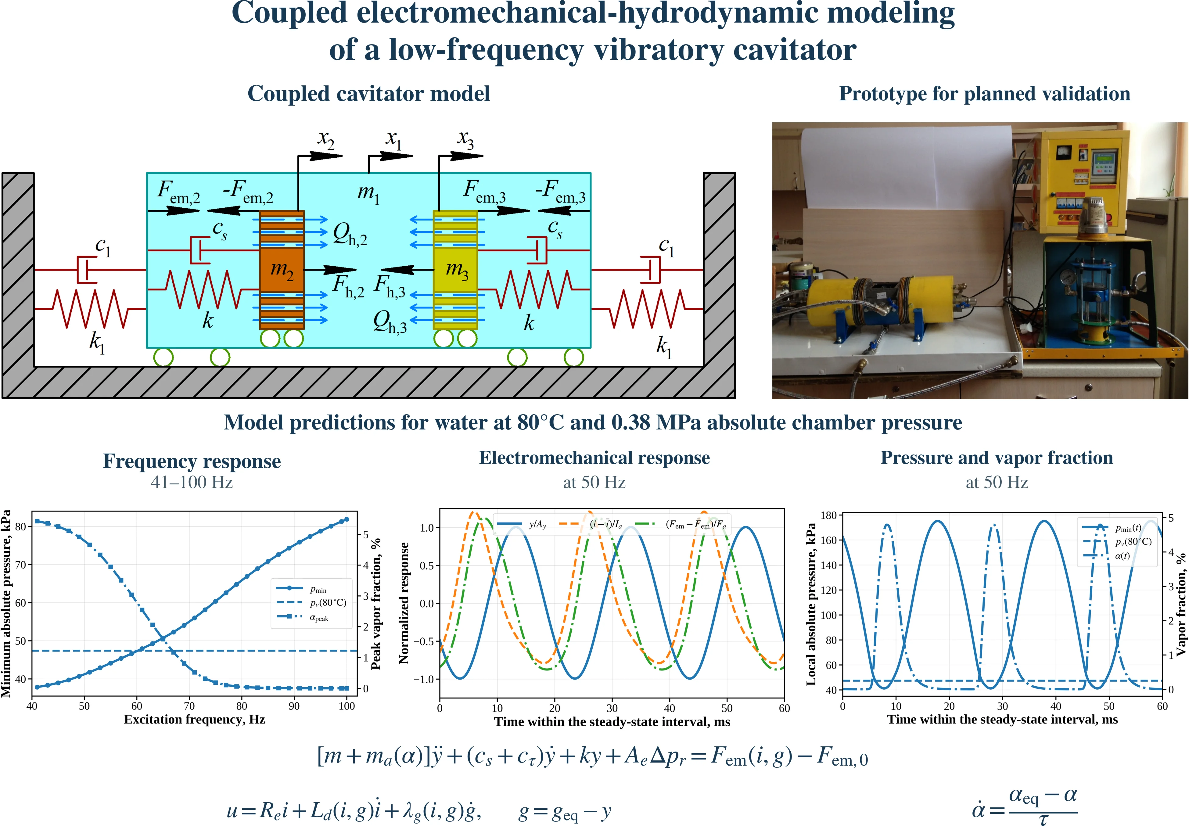
Highlights
- A coupled model links variable-gap electromagnetic drives, grate motion, nonlinear hydraulic loading and finite-rate vapor-fraction evolution.
- For water at 80°C and 0.38 MPa absolute chamber pressure, the model predicts pressure-threshold crossing over approximately 41-60 Hz.
- At 50 Hz, simulations predict a 2.21 mm grate amplitude, 41.2 kPa minimum local pressure and 4.8% peak vapor fraction.
- At 50 Hz, predicted current and force lags relative to voltage are 29.6° and 59.7°, showing the limitations of prescribed in-phase harmonic excitation.
- At 50 Hz, predicted electrical input to both drives is approximately 0.65 kW, with equivalent hydrodynamic damping of 138 N·s/m per moving assembly.
1. Introduction
Hydrodynamic cavitation is increasingly applied to water and wastewater treatment because cavity collapse intensifies mixing and physicochemical degradation. Reviews [1]-[3] summarize advanced-oxidation mechanisms, reactor configurations, pollutant removal, and energy-efficiency constraints. For perforated restrictions, Maynes et al. [4] and Malavasi et al. [5] showed that head loss and cavitation inception depend on the free-area ratio, hole geometry, plate thickness, and Reynolds number. Ezoji et al. [6] demonstrated that oscillating perforated plates exhibit amplitude-dependent added mass and nonlinear damping.
Electromagnetic oscillators must be modeled jointly with their mechanical load. Hung and Lim [7] experimentally confirmed the influence of voltage and air gap on current, force, and plunger displacement, whereas Naseradinmousavi and Nataraj [8] formulated nonlinear actuator dynamics with position-dependent inductance. The Rayleigh-Plesset equation [9] remains the classical basis for reduced bubble-growth and collapse descriptions. Aftanaziv et al. [10] developed an electromagnetic vibratory cavitator for low-frequency liquid treatment.
The authors’ previous study [11] proposed a continuous-flow device with two oppositely moving perforated grates, but prescribed the electromagnetic forces harmonically and represented liquid loading by generalized viscous damping. A recent hydrodynamic-cavitation generator driven by a linear electromagnetic piston [12] further demonstrates the relevance of coupled actuator-fluid analysis. However, a compact model combining a variable-gap electromagnetic drive, oscillating perforated-grate hydrodynamics, and finite-rate vapor-content evolution has not yet been developed for the considered continuous-flow cavitator. The present study therefore evaluates the effects of excitation frequency on grate motion, local pressure, vapor content, current, power demand, and hydraulic dissipation.
Experimental studies involving Aftanaziv and co-workers have investigated vibrocavitation of brewing wastewater [13], frequency-dependent treatment of model contaminated water [14], and gas-assisted ultrasonic treatment of fat-and-oil-plant wastewater [15]. These studies establish relevant treatment experience, but do not validate the dynamic predictions of the present device. Accordingly, the discussion below distinguishes existing experimental evidence from planned model validation and examines the changes required for viscous and non-Newtonian liquids.
2. Research methodology
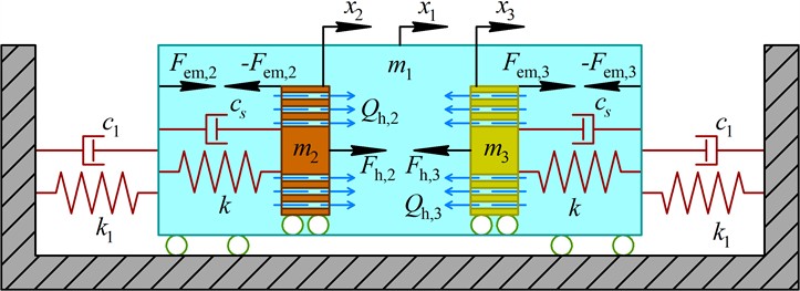
The computational diagram of the cavitator is shown in Fig. 1. The body of mass is connected to the stationary base by the stiffness and damping , whereas two identical armature-rod-grate assemblies are connected to the body by elastic and dissipative elements and . The electromagnetic drives act in opposite global directions. The absolute displacements , , and are shown in Fig. 1. The local displacements of the moving assemblies toward the corresponding stators are defined as and . Under the synchronous symmetric operating conditions considered in Section 3 of this research, the local motions satisfy , while the global grate motions are antiphase and their dynamic reactions on the cavitator body are mutually compensated. Therefore, both moving assemblies can be represented by one local coupled subsystem.
Fig. 1Computational diagram of the coupled cavitator model: m1 – cavitator body; m2, m3 – armature-rod-grate assemblies; x1, x2, x3 – absolute displacements; Fem,j and Fh,j – electromagnetic and hydrodynamic forces; Qh,j – liquid flow rates through the perforated grates
The reduced mechanical equation is written as:
where the relative flow rate through the perforated grate, nonlinear pressure-loss increment, added liquid mass, and mixture properties are:
Eq. (2) accounts for hydraulic inertance, linear and quadratic losses, and the dependence of the liquid-vapor mixture properties on the instantaneous vapor fraction. The electromagnetic subsystem is voltage-driven and includes the variable air gap, magnetic saturation, and motion-induced electromotive force:
where , , and the static magnetic force is balanced by the initial spring preload.
For long-term frequency-response simulations, the cavitation dynamics are represented by a regularized pressure-based vapor-fraction model:
where, is the pressure-dependent equilibrium vapor fraction, controls the smoothness of the cavitation transition, and and are effective vapor-cloud growth and collapse times, respectively. Eq. (4) is a phenomenological reduced-order closure rather than a direct integration of the Rayleigh-Plesset equation [9].
All pressures in Eq. (4) are absolute. Because the regularized closure introduces a smooth transition, the condition is used only as a pressure-based indicator that the cavitation threshold has been crossed, rather than as a discontinuous phase-change criterion.
The adopted magnetic, hydraulic, and vapor-fraction coefficients require experimental identification for the present device. The calculations below therefore constitute model predictions; numerical solver agreement does not establish experimental validity.
3. Results and discussion
3.1. Numerical response for water purification process
Numerical simulation was performed for the coupled electromechanical-hydrodynamic model derived in Section 2. The calculations were implemented in Python 3.13.5 using NumPy 2.3.5 and SciPy 1.17.0. The reported results were obtained using the implicit Radau solver, while selected operating points were recalculated with the BDF method to verify numerical consistency. The maximum integration step was restricted to approximately one hundredth of the excitation period. Each frequency case was simulated for at least 35 oscillation cycles or 0.70 s, whichever was longer, and only the final eight cycles were used to calculate steady-state amplitudes, root-mean-square values, phase shifts, and mean powers.
The processing temperature and pressure selected in Table 1 correspond to the operating range proposed for the cavitator, namely approximately 75-80°C and 0.35-0.40 MPa. In the present simulations, the chamber pressure 0.380 MPa was interpreted as an absolute pressure. The quantities , , , and were calculated from the corresponding geometric and electrical parameters. Frequencies below 41 Hz were excluded because the predicted minimum air gap approached the imposed limit 0.8 mm, indicating the onset of electromagnetic pull-in or mechanical contact beyond the validity of the no-contact model.
Table 1Parameters adopted for the numerical simulation
Symbol | Value | Unit | Symbol | Value | Unit |
29.5 | kg | 3.55×10⁻⁴ | Pa·s | ||
0.85 | kg | 7.854×10⁻³ | M2 | ||
1.9×10⁴ | N/m | 4.241×10⁻⁴ | m2 | ||
50 | N·s/m | 0.054 | – | ||
8.8×10⁴ | N/m | 1.5 | – | ||
55 | N·s/m | 6.0×10⁻³ | M3/s (21.6 m3/h) | ||
, | 5.0; 0.8 | mm | 0.15 | – | |
0.8 | mm | 1.8 | – | ||
700 | – | 1.0×10⁶ | Pa·s/m3 | ||
2.0×10⁻³ | m² | 0.012 | m | ||
4.5 | A | 0.010 | m | ||
0.012 | H | 2.8 | – | ||
35 | Ω | 1.5×10⁻³ | M2 | ||
, | 84; 140 | V | 20 | N·s/m | |
2.40 | A | 0.06 | – | ||
98.84 | N | 2.5 | – | ||
80 | °C | 4.0 | kPa | ||
0.380 | MPa (abs.) | 0.5; 1.5 | ms | ||
, | 971.8; 0.293 | kg/m³ | 41-100 | Hz | |
47.4 | kPa | 0 | m | ||
, | 100; 4.5 | mm | 0 | m/s | |
60 | – | 2.4 | A | ||
3.0 | mm | 0 | – |
Fig. 2(a) shows the dependence of the minimum local absolute pressure and maximum vapor volume fraction on the excitation frequency. At 41 Hz, the minimum pressure decreases to 37.84 kPa, which is 9.56 kPa below the saturated vapor pressure of water at 80 °C. The corresponding maximum vapor fraction is 5.43 %. At 50 Hz, the minimum pressure equals 41.20 kPa and the maximum vapor fraction reaches 4.79 %.
The pressure-threshold crossing occurs at approximately 60-61 Hz. At 59 Hz, the minimum pressure is 46.64 kPa, whereas at 61 Hz it rises to 47.93 kPa. Above this range, the instantaneous pressure no longer falls below , although a small modeled vapor fraction remains because the regularized closure in Eq. (4) gives a nonzero equilibrium fraction above the saturation pressure; finite relaxation additionally produces phase lag. At frequencies above approximately 78-80 Hz, the maximum vapor fraction becomes lower than 0.1 %. At 100 Hz, the predicted value is only 8.9×10⁻⁴%, and cavitation is practically absent.
These results indicate that the cavitation intensity is governed not only by the nominal liquid-flow rate but also by the grate velocity and acceleration. The lower-frequency operating regime generates larger volumetric displacement of liquid through the holes and a stronger inertial pressure reduction. Thus, the enhanced mathematical model additionally identifies an approximate pressure-based cavitation interval of 41-60 Hz for the adopted parameter set.
Fi2(b) presents the electromechanical response at 50 Hz. In Fig. 2(b), , , and denote the half peak-to-pg. eak amplitudes of the displacement, current, and electromagnetic force, respectively, while overbars indicate cycle-averaged values. Although the strongest pressure reduction is predicted near 41 Hz, the corresponding grate amplitude reaches approximately 3.04 mm and the minimum air gap decreases to about 1.13 mm. At 50 Hz, the minimum instantaneous gap increases to approximately 2.59 mm, providing a margin of approximately 1.79 mm above the imposed lower limit mm. The steady-state displacement amplitude is 2.205 mm, the root-mean-square grate velocity is 0.491 m/s, and the maximum acceleration is 221.1 m/s2, or approximately 22.54.
The instantaneous coil current varies from 0.70 to 5.00 A, and its root-mean-square value is 2.81 A. The electromagnetic force changes from approximately 9.3 to 270.7 N. However, the fundamental harmonic of this force has an amplitude of only approximately 133.5 N. Therefore, the maximum instantaneous force must not be used as an equivalent amplitude of an ideal sinusoidal excitation.
Frequency-domain analysis of the steady-state signals gives the following phase shifts relative to the applied voltage: –29.6°, –59.7°, –149.8°. The substantial current and force phase lags confirm that the electromagnetic drive cannot be represented adequately by a mechanical force that is assumed to be perfectly synchronized with the supply voltage.
The calculated mean electrical input power is 322.7 W per coil. The corresponding copper loss is 276.2 W, while approximately 46.5 W is converted into mechanical power. The corresponding model-based electromechanical conversion efficiency is approximately 14.4 % per drive, excluding losses in the power converter. For two identical electromagnetic drives, the total electrical input is therefore approximately 645 W. Of the mechanical power delivered to each moving assembly, approximately 33.3 W is dissipated through the modeled hydraulic resistance and 13.3 W through structural damping.
The hydrodynamic-force amplitude, evaluated as one-half of its peak-to-peak range, is approximately 99.4 N at 50 Hz. Its fundamental harmonic is shifted by approximately 174.5° relative to the grate velocity and therefore acts predominantly as a damping force. The corresponding equivalent linear hydrodynamic damping evaluated from the fundamental components is approximately 138 N·s/m. Together with the assumed structural damping of 55 N·s/m, this gives approximately 193 N·s/m.
Fig. 2Predicted responses of the coupled model
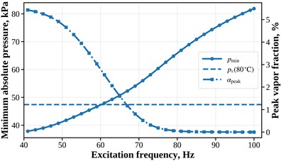
a) Frequency dependence of the minimum local pressure and maximum vapor volume fraction
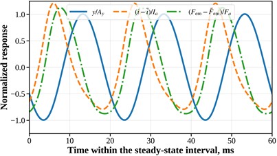
b) Normalized steady-state displacement, coil current, and electromagnetic force at 50 Hz
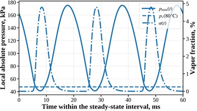
c) Local absolute pressure and vapor volume fraction during three steady-state oscillation cycles at 50 Hz
As shown in Fig. 2(c), at 50 Hz, the local absolute pressure varies from approximately 41.2 to 175.2 kPa. The pressure remains below the saturated vapor pressure for approximately 15.8 % of each oscillation period. Due to the finite vapor-cloud collapse time, the vapor fraction remains above 1 % for approximately 30.4 % of the period.
The vapor fraction reaches its maximum after the instant of minimum pressure rather than simultaneously with it. This phase delay reflects the finite rate of vapor-cloud development.
The mean velocity through the grate holes is approximately 14.15 m/s and varies from 12.28 to 16.16 m/s during the cycle. The corresponding hole Reynolds number, , varies approximately within 1.01×10⁵ 1.33×10⁵, confirming strongly turbulent through-hole flow and supporting the use of a quadratic pressure-loss term.
4. Experimental evidence and planned validation
Shevchuk et al. [13] experimentally investigated brewing yeast-containing wastewater using an electromagnetic vibratory cavitator and found that combined vibrocavitation and nitrogen treatment improved biological and organic decontamination. Aftanaziv et al. [14] measured chemical oxygen demand during low-frequency vibrocavitation of model contaminated water. For the reported uric-acid-to-water ratio of 1:10 under nitrogen, organic-contaminant destruction after one hour reached 70 %, 84 %, and 75 % at 25, 37, and 75 Hz, respectively. These published results demonstrate that treatment performance depends on excitation frequency, but the 37 Hz optimum for that apparatus cannot be transferred to the present geometry and operating conditions.
Vashkurak et al. [15] measured chemical oxygen demand and microbial counts during ultrasonic treatment of fat-and-oil-plant wastewater in different gas environments, demonstrating the influence of gas composition on treatment efficiency. That study concerns aqueous wastewater and ultrasonic cavitation; it is not an experiment on pure oil or on the present low-frequency drive. Collectively, these studies support the technological feasibility of cavitation treatment, but their process-level measurements cannot establish the accuracy of the displacement, current, local pressure, or vapor-fraction predictions reported here.
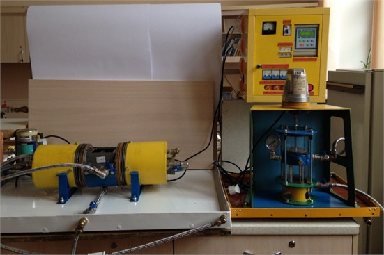
The theoretical predictions developed in this article will undergo dedicated experimental validation in subsequent research using the laboratory equipment developed at Lviv Polytechnic National University (see Fig. 3). Synchronized measurements of grate displacement, coil voltage and current, chamber pressure, local pressure near the holes, flow rate, and temperature will be compared with predicted amplitudes, phases, pressure minima, and mean electrical power. Optical observations will assess cavity onset and cloud timing; quantitative vapor-fraction validation will require a calibrated measurement method. Parameters will be identified using a subset of operating points and tested at separate frequencies, with repeated measurements and uncertainty estimates. Water tests will precede investigations of viscous and non-Newtonian liquids.
Fig. 3Experimental prototype of the vibratory cavitator
5. Numerical response for water purification process
The present predictions apply to water at 80 °C. For illustration, the adopted mean flow rate and hole geometry give a mean hole velocity of 14.15 m/s. A hypothetical Newtonian oil with density 850 kg/m3 and dynamic viscosity 0.10 Pa·s at its operating temperature would have a mean hole Reynolds number of approximately 361 at the same imposed flow rate, compared with approximately 1.16×10⁵ for water. These are scaling estimates, not additional simulations. Low Reynolds number does not itself exclude cavity formation: experiments comparing water and oil in the same nozzle reported cavities in laminar oil flow and showed the importance of released noncondensable gas [16].
In the present formulation, viscosity enters the hydraulic load through coefficients that are held fixed for the water calculations; changing only the tabulated viscosity would therefore not predict its effect on motion. For viscous Newtonian liquids, linear hydraulic resistance and shear-related damping must depend on viscosity, and the loss and local-pressure coefficients must be identified for the appropriate flow regime. Higher viscosity increases viscous dissipation at prescribed motion and generally attenuates motion near resonance, but displacement, phase shifts, and pressure minima require recalculation of the coupled system. The outcome also depends on whether flow rate or available pumping pressure is maintained. The short holes require allowance for entrance losses and unsteady flow. Density, viscosity, and vapor pressure must correspond to the operating temperature. For oils, gas release must be distinguished from vapor formation; a separate gas-content description is needed where degassing is significant [16].
For many non-Newtonian liquids, apparent viscosity depends on shear rate, while yield stress or viscoelasticity may introduce additional effects. Shear thinning can reduce local viscous resistance relative to that estimated using zero-shear viscosity, whereas shear thickening can increase it. Experiments on shear-thickening suspensions demonstrate that rheology also changes bubble deformation and collapse [17]. A measured constitutive law, such as Carreau-Yasuda for shear thinning or Herschel-Bulkley for yield-stress behavior, must therefore be incorporated into the hydraulic-load description; significant viscoelasticity requires stress evolution as well. The vapor-fraction closure and its growth and collapse times must also be reassessed. Consequently, neither the predicted 41-60 Hz pressure-threshold interval nor the operating compromise near 50 Hz can be assumed valid for other fluids without further modeling and experiments.
6. Conclusions
A compact coupled electromechanical-hydrodynamic model of the low-frequency cavitator has been developed. The formulation accounts for the variable air gap, magnetic saturation, motion-induced electromotive force, liquid added mass, nonlinear pressure losses, and finite-rate vapor-content evolution. For the adopted parameter set, the model predicts a pressure-based cavitation interval of approximately 41-60 Hz, whereas cavitation becomes practically negligible at 100 Hz. At 50 Hz, the predicted grate amplitude is 2.21 mm, the minimum local pressure is 41.2 kPa, the peak vapor fraction is 4.8 %, the maximum acceleration reaches approximately 22.5g, and the RMS coil current is 2.81 A. The current and electromagnetic-force phase lags relative to the voltage are approximately 29.6° and 59.7°, confirming that representation of the electromagnetic excitation by a prescribed in-phase harmonic force is inadequate. The predicted total electrical input to the two drives is approximately 0.65 kW, while the dissipative component of the hydrodynamic load corresponds to an equivalent damping of about 138 N·s/m. Compared with the previous force-driven model [11], the predicted 50 Hz displacement amplitude is approximately 21 % lower because the actual fundamental electromagnetic-force amplitude is limited by current dynamics, variable air gap, and magnetic saturation. Thus, operation near 50 Hz appears to provide a practical compromise between pressure reduction, grate displacement, and air-gap safety for the adopted parameter set.
Published experiments on related cavitation devices support the feasibility of the treatment principle, while direct quantitative validation of the present coupled model remains to be performed. The theoretical predictions will be experimentally tested in subsequent research. Application to viscous oils and non-Newtonian liquids requires fluid-specific hydraulic coefficients, appropriate rheological relations, and reassessment of the vapor and gas dynamics.
References
-
M. Gągol, A. Przyjazny, and G. Boczkaj, “Wastewater treatment by means of advanced oxidation processes based on cavitation – a review,” Chemical Engineering Journal, Vol. 338, pp. 599–627, Jan. 2018, https://doi.org/10.1016/j.cej.2018.01.049
-
Y. Chen, C. Yin, and Y. Song, “Application of hydrodynamic cavitation in the field of water treatment,” Chemical Papers, Vol. 77, No. 7, pp. 3521–3546, Mar. 2023, https://doi.org/10.1007/s11696-023-02754-y
-
A. V. Mohod, A. C. S. C. Teixeira, M. V. Bagal, P. R. Gogate, and R. Giudici, “Degradation of organic pollutants from wastewater using hydrodynamic cavitation: a review,” Journal of Environmental Chemical Engineering, Vol. 11, No. 3, p. 109773, Mar. 2023, https://doi.org/10.1016/j.jece.2023.109773
-
D. Maynes, G. J. Holt, and J. Blotter, “Cavitation inception and head loss due to liquid flow through perforated plates of varying thickness,” Journal of Fluids Engineering, Vol. 135, No. 3, Mar. 2013, https://doi.org/10.1115/1.4023407
-
S. Malavasi, G. V. Messa, U. Fratino, and A. Pagano, “On cavitation occurrence in perforated plates,” Flow Measurement and Instrumentation, Vol. 41, pp. 129–139, Nov. 2014, https://doi.org/10.1016/j.flowmeasinst.2014.11.002
-
M. Ezoji, N. Shabakhty, and L. Tao, “Hydrodynamic damping of solid and perforated heave plates oscillating at low KC number based on experimental data: a review,” Ocean Engineering, Vol. 253, p. 111247, Apr. 2022, https://doi.org/10.1016/j.oceaneng.2022.111247
-
N. B. Hung and O. T. Lim, “A simulation and experimental study on the operating characteristics of a solenoid gas injector,” Advances in Mechanical Engineering, Vol. 11, No. 1, pp. 1–14, Jan. 2019, https://doi.org/10.1177/1687814018817421
-
P. Naseradinmousavi and C. Nataraj, “Nonlinear mathematical modeling of butterfly valves driven by solenoid actuators,” Applied Mathematical Modelling, Vol. 35, No. 5, pp. 2324–2335, Nov. 2010, https://doi.org/10.1016/j.apm.2010.11.036
-
M. S. Plesset, “The dynamics of cavitation bubbles,” Journal of Applied Mechanics, Vol. 16, No. 3, pp. 277–282, Sep. 1949, https://doi.org/10.1115/1.4009975
-
I. Aftanaz, “Electromagnetic vibratory cavitator,” Przegląd Elektrotechniczny, Vol. 1, No. 4, pp. 26–31, Apr. 2019, https://doi.org/10.15199/48.2019.04.05
-
I. Aftanaziv, V. Korendiy, O. Kachur, O. Strogan, I. Svidrak, and R. Stotsko, “Design peculiarities and mathematical model of an enhanced low-frequency vibratory cavitation device,” Vibroengineering Procedia, Vol. 51, pp. 1–7, Oct. 2023, https://doi.org/10.21595/vp.2023.23577
-
J. Gostiša et al., “Design and development of a novel magnetic generator of hydrodynamic cavitation,” Results in Engineering, Vol. 29, p. 109903, Mar. 2026, https://doi.org/10.1016/j.rineng.2026.109903
-
L. Shevchuk, I. Aftanaziv, and T. Falyk, “Vibrocavitation decontamination of brewing yeast-containing wastewater,” Chemistry and Chemical Technology, Vol. 11, No. 4, pp. 475–479, 2017, https://doi.org/10.23939/chcht11.04.475
-
I. Aftanaziv, L. Shevchuk, M. Malovanyy, L. Strutynska, and I. Samsin, “Cavitation-reagent technology for water purification of pools and water parks,” Journal of Ecological Engineering, Vol. 20, No. 6, pp. 141–152, Jun. 2019, https://doi.org/10.12911/22998993/108638
-
U. Vashkurak, L. Shevchuk, I. Nykulyshyn, and I. Aftanaziv, “Research into effectiveness of cavitation cleaning of wastewater of a fat-and-oil plant from organic and biological contamination in the presence of various gases,” Eastern-European Journal of Enterprise Technologies, Vol. 3, No. 10 (93), pp. 51–58, 2018, https://doi.org/10.15587/1729-4061.2018.131953
-
J. Jablonská, M. Kozubková, and M. Bojko, “Flow of oil and water through the nozzle and cavitation,” Processes, Vol. 9, No. 11, p. 1936, Oct. 2021, https://doi.org/10.3390/pr9111936
-
G. T. Bokman, O. Supponen, and S. A. Mäkiharju, “Cavitation bubble dynamics in a shear-thickening fluid,” Physical Review Fluids, Vol. 7, No. 2, Feb. 2022, https://doi.org/10.1103/physrevfluids.7.023302
About this article

The authors have not disclosed any funding.
The datasets generated during and/or analyzed during the current study are available from the corresponding author on reasonable request.
Prof. Vitaliy Korendiy is a chair of the 78th International Conference on Vibroengineering and was not involved in the editorial review and/or the decision to publish this article.

