Abstract
This study proposes a domain-decomposed physics-informed neural network method for identifying piecewise moving heat-flux boundary conditions in thermite-induced transient heat transfer. The axial domain is divided into three subdomains, each with an independent heat-flux profile and propagation speed. The local heat-flux profiles are parameterized using radial basis functions and identified from outer-wall temperature measurements. Interface continuity conditions are imposed to ensure physical consistency between adjacent subdomains. Numerical results show that the proposed method can recover the main features of the piecewise heat-flux profiles and identify the local propagation speeds with relative errors within approximately 5 %. The method provides a flexible framework for describing locally non-uniform moving thermal inputs.
1. Introduction
Inverse heat conduction problems aim to infer unknown thermal boundary conditions, material parameters, or heat-source distributions from limited temperature measurements. They are widely encountered in thermal protection, energy engineering, and thermal diagnostics. However, transient inverse heat conduction problems are often ill-posed, especially when the unknown thermal input varies in both space and time. Physics-informed neural networks (PINNs) provide a promising approach for such problems by incorporating governing equations and boundary conditions into the training loss [1].
PINNs have been increasingly applied to inverse heat transfer problems. Haghighat and Juanes [2] introduced SciANN as an open-source framework for physics-informed learning and scientific computing. Liu et al. [3] used PINNs to identify surface heat flux and moving ablation-boundary evolution from temperature measurements. Cai et al. [4] estimated surface heat flux from measured surface temperature fields using a PINN framework. Hazra et al. [5] applied PINNs to infer convective heat transfer coefficients in jet impingement cooling. Bidou et al. [6] investigated inverse heat conduction problems involving moving heat sources. Zhao et al. [7] reviewed recent developments of PINNs in heat-transfer-dominated multiphysics systems. These studies demonstrate the potential of PINNs for solving inverse heat transfer problems with limited measurements.
In thermite-based wellbore plugging and abandonment, the heat released by the thermite reaction propagates along the axial direction and induces a strong transient thermal response in the surrounding tube wall. Shang et al. [8] proposed a PINN-based method to identify this moving heat-flux boundary condition from outer-wall temperature measurements. In that formulation, the heat input was described by a fixed heat-flux profile moving axially with a single propagation speed, which is consistent with the shifted heat-flux behavior observed by Dourado da Silva et al. [9]. This model can effectively capture the overall propagation feature of the thermite-induced heat input.
Nevertheless, in practical thermite reactions, the combustion state, powder distribution, and local heat-transfer conditions may vary along the axial direction. Therefore, the heat-flux intensity and propagation speed may not remain uniform over the entire domain. To enable the simultaneous identification of distinct heat-flux profiles and propagation speeds in different regions, this study adopts an XPINN-based domain-decomposition framework. The axial domain is divided into three subdomains, and each subdomain is assigned an independent heat-flux profile and propagation speed. Temperature and heat-flux continuity conditions are imposed at the internal interfaces, leading to a domain-decomposed PINN method for identifying piecewise moving heat-flux boundary conditions.
2. Research method
2.1. Problem description
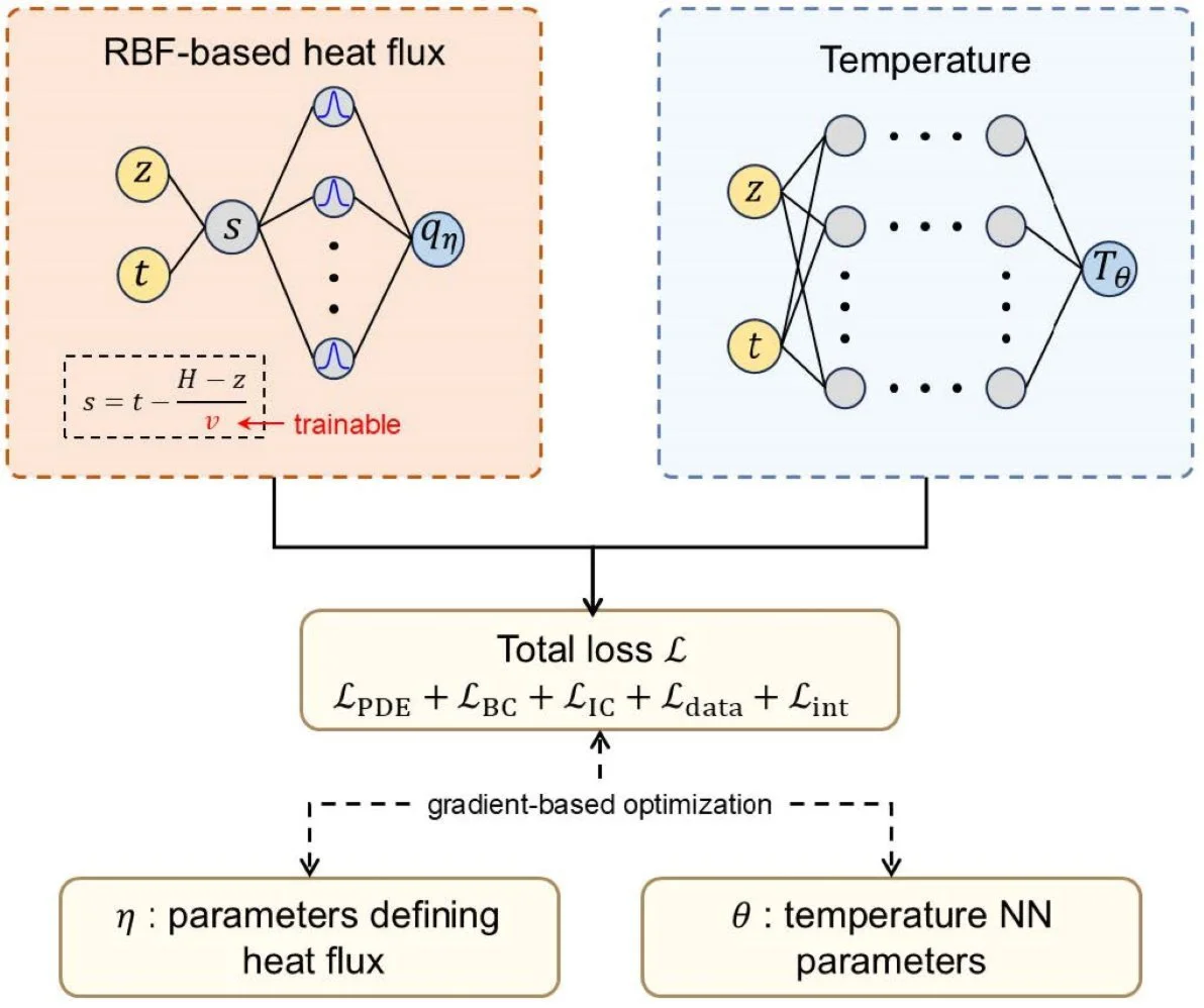
This study considers the identification of moving heat-flux boundary conditions in a tubular metallic structure. The physical model is based on a typical thermite-heating configuration, as shown in Fig. 1. The heat released by the thermite reaction is represented as an equivalent moving heat-flux boundary condition applied to the inner wall of the tube. Several temperature sensors are placed on the outer wall at 0.84, 0.64, 0.52, 0.32, 0.20, and 0.0 m to measure the transient thermal response. The inverse problem aims to recover the inner-wall moving heat flux and its propagation speed from these outer-wall temperature measurements.
For the conventional moving heat-flux model, the boundary heat flux can be expressed as:
where denotes the heat-flux profile in the moving coordinate, is the shifted time coordinate, is the axial length of the computational domain, is the axial coordinate, and is the propagation speed of the moving heat flux. This formulation indicates that the heat-flux histories at different axial locations have similar temporal shapes but are shifted in time according to the propagation speed.
To account for local differences in heat release, the computational domain is divided into three axial subdomains:
In each subdomain, an independent heat-flux profile and propagation speed are introduced:
where and denote the heat-flux profile and propagation speed in the -th subdomain, respectively. denotes the arrival time at the top of the -th subdomain. In this way, the original single moving heat-flux identification problem is extended to a piecewise moving heat-flux identification problem.
The axisymmetric transient heat conduction problem is described by Eq. (4):
where, denotes the computational domain, is the inner-wall heat-flux boundary, and denote the top and bottom boundaries, respectively.
2.2. Domain-decomposed PINN for heat-flux boundary identification
Since the wall thickness is much smaller than the axial length and the radial heat diffusion in the metallic tube is relatively fast, a one-dimensional effective heat conduction model is adopted in the inverse analysis to reduce the computational cost. The effective governing equation is written as:
where and are effective geometric factors determined by the inner and outer radii of the tube:
In this effective model, the unknown inner-wall heat flux appears explicitly in the governing equation. To make it trainable within the PINN framework, the heat-flux profile in each subdomain is parameterized using radial basis functions:
where , , and are the weight, center, and width of the -th radial basis function in the -th subdomain, respectively. These quantities are treated as trainable parameters. The propagation speed in each subdomain is also identified during the optimization process.
Fig. 1Domain-decomposed tubular model with piecewise moving heat flux
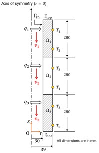
Fig. 2Framework of the domain-decomposed PINN method
The temperature field is approximated by a neural network . The required temporal and spatial derivatives are obtained through automatic differentiation, which allows the governing-equation residual to be constructed directly. During training, the governing equation, boundary conditions, initial condition, and temperature measurements are combined into a unified loss function. The trainable parameters of the temperature network and the heat-flux representation are updated simultaneously through gradient-based optimization. The overall framework is shown in Fig. 2.
Specifically, the governing-equation residual, boundary-condition loss, initial-condition loss, and data loss are defined in Eq. (8):
The total loss function is written as:
where , , , and are the weighting coefficients of the corresponding loss terms. To maintain physical consistency between adjacent subdomains, the interface loss penalizes discontinuities in both temperature and heat flux.
3. Results and discussion
To evaluate the proposed method, a numerical case with piecewise moving heat-flux boundary conditions was constructed. The computational domain was divided into three axial subdomains, and different reference heat-flux profiles and propagation speeds were assigned to these subdomains. The outer-wall temperature histories were generated from forward simulations and used as measurement data for the inverse identification. Training was performed on an NVIDIA GeForce RTX 4070 Ti SUPER GPU using Adam with a constant learning rate of 0.0001. The model was trained for 40,000 iterations, with a total training time of approximately 32.84 min. The training history of the total loss is shown in Fig. 3.
Fig. 4 shows the temperature fitting results and the recovered heat-flux profiles. The predicted temperature histories agree well with the reference data at the measurement locations, indicating that the transient thermal response of the tube wall is properly reconstructed. The recovered heat-flux profiles also capture the main features of the reference profiles in the three subdomains, including the peak locations and overall temporal shapes. Minor discrepancies remain near the peaks of the recovered heat-flux profiles. In addition, thermal diffusion smooths the temperature response, making sharp heat-flux peaks more difficult to recover.
Fig. 3Training history of the total loss
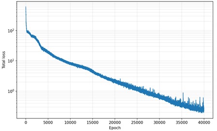
Fig. 4Temperature fitting and heat-flux identification results
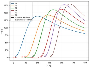
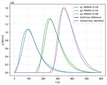
The propagation speeds in the three subdomains were also identified. The reference speeds were 2.000, 3.000, and 4.000 mm/s, while the identified values were 2.097, 3.145, and 4.180 mm/s, corresponding to relative errors of 4.86 %, 4.82 %, and 4.50 %, respectively. These results show that the proposed method can reasonably identify the local propagation speeds of the moving heat-flux boundary.
To assess robustness, Gaussian noise at levels of 1 %, 3 %, and 5 % was added to all measured temperature histories. The results at 1 % noise were comparable to those obtained from the noise-free data. Higher noise levels increased the identification errors, particularly for the propagation speeds, while the recovered heat-flux profiles were less affected.
Overall, the domain-decomposed PINN can identify both the piecewise heat-flux profiles and their corresponding propagation speeds. Compared with the single-profile and single-speed formulation, the proposed method provides a more flexible description of locally non-uniform moving heat inputs.
4. Conclusions
A domain-decomposed PINN method was developed for identifying piecewise moving heat-flux boundary conditions from outer-wall temperature measurements. By dividing the axial computational domain into three subdomains, the proposed method allows each subdomain to have an independent heat-flux profile and propagation speed, thereby extending the conventional single-profile moving heat-flux model.
Numerical results show that the proposed method can reproduce the measured temperature histories and recover the main characteristics of the heat-flux profiles in different subdomains. The identified propagation speeds also agree well with the reference values, with relative errors within approximately 5%. These results demonstrate the feasibility of the proposed method for describing locally non-uniform moving heat inputs in thermite-induced transient heat transfer problems.
However, the present numerical example demonstrates the method’s feasibility using temperature data without added noise. Future work will evaluate its robustness using noisy temperature data to better reflect practical measurement conditions.
References
-
M. Raissi, P. Perdikaris, and G. E. Karniadakis, “Physics-informed neural networks: A deep learning framework for solving forward and inverse problems involving nonlinear partial differential equations,” Journal of Computational Physics, Vol. 378, pp. 686–707, Nov. 2018, https://doi.org/10.1016/j.jcp.2018.10.045
-
E. Haghighat and R. Juanes, “SciANN: A Keras/TensorFlow wrapper for scientific computations and physics-informed deep learning using artificial neural networks,” Computer Methods in Applied Mechanics and Engineering, Vol. 373, p. 113552, Nov. 2020, https://doi.org/10.1016/j.cma.2020.113552
-
L. Liu, Y. Liang, Y. Shang, and D. Liu, “Identification of ablation surface evolution using physics-informed neural network,” International Communications in Heat and Mass Transfer, Vol. 167, p. 109310, Jul. 2025, https://doi.org/10.1016/j.icheatmasstransfer.2025.109310
-
Z. Cai, X. Lin, and T. Liu, “Physics-informed neural network for estimating surface heat flux from surface temperature measurements,” International Journal of Heat and Mass Transfer, Vol. 253, p. 127580, Jul. 2025, https://doi.org/10.1016/j.ijheatmasstransfer.2025.127580
-
A. Hazra, P. Sarkar, and S. Sarkar, “PINN-based estimation of convective heat transfer in jet impingement cooling,” Applied Thermal Engineering, Vol. 284, p. 129088, Nov. 2025, https://doi.org/10.1016/j.applthermaleng.2025.129088
-
M. S. Bidou, J.-G. Bauzin, and N. Laraqi, “Physics-informed neural networks for 2D-transient inverse heat conduction problem involving static and moving heat source,” International Journal of Heat and Mass Transfer, Vol. 259, p. 128349, Jan. 2026, https://doi.org/10.1016/j.ijheatmasstransfer.2026.128349
-
Z. Zhao, Y. Wang, W. Zhang, Z. Ba, and L. Sun, “Physics-informed neural networks in heat transfer-dominated multiphysics systems: A comprehensive review,” Engineering Applications of Artificial Intelligence, Vol. 157, p. 111098, Jun. 2025, https://doi.org/10.1016/j.engappai.2025.111098
-
Y. Shang, D. Liu, and H. Wu, “Identification of a moving heat-flux boundary condition in thermite-based wellbore plugging and abandonment with physics-informed neural networks,” International Journal of Heat and Mass Transfer, Vol. 267, p. 129004, May 2026, https://doi.org/10.1016/j.ijheatmasstransfer.2026.129004
-
R. G. Dourado Da Silva, E. S. Magalhães, and L. C. M. Pires, “Estimation of thermal input in thermite reaction for innovative wellbore plugging and abandonment techniques,” International Communications in Heat and Mass Transfer, Vol. 148, p. 107071, 2023, https://doi.org/10.1016/j.icheatmasstransfer.2023.107071
About this article

Supported by Project “Vice President of Science and Technology” of Changping District, Beijing, No. 202402004009.
The datasets generated during and/or analyzed during the current study are available from the corresponding author on reasonable request.
The authors declare that they have no conflict of interest.

