Machine learning-based predictive modeling for surface roughness in abrasive machining

1. Introduction

Machining has been a crucial element of the production industry for the production of spares, tools, equipment, etc., of very high precision and quality. Surface Grinding (SG) is generally the last step of machining, performed to impart the necessary functional features such as close tolerances in dimensions and a good surface finish [1-3]. The surface roughness (Ra) is one of the significant parameters of performance that is required to be monitored throughout the surface grinding operation, which also signifies the finishing quality of the machined parts [4-6]. The input parameters that significantly affect the grinding output response Ra include the Cutting Fluid (CF), Grinding Wheel Grade (GWG), Grinding Wheel Speed (GWS), Work Speed (WS), and Depth of Cut (DOC), etc. [4], [7]. So, the selection of optimal grinding settings becomes necessary to achieve the desired Ra during the grinding operation [8], [9]. The machinists generally use the trial-and-error strategy to decide these input settings to get the desired surface finish. This trial-and-error approach is not so efficient, time-consuming, and wasteful of resources. Going through the literature, it is observed that the Taguchi experimental design method is generally used along with other optimization methods such as Grey Relational Analysis (GRA), Response Surface Methodology (RSM), etc., to decide the optimal grinding input settings. The development of Machine Learning (ML) predictive models also offers a solution for this problem. Here, there is a scope to alter the settings and predict the response before the actual grinding operation is performed [10].

The other challenge associated with grinding operation is the generation of intense heat at the time of grinding and the induction of thermal stresses hampering the surface finish, dimensional accuracy, grain structure, and mechanical properties of the ground workpiece [11-13]. The use of a CF is the general practice to control this problem, which provides proper lubrication and cooling, resulting in an improved surface finish [14], [15]. Petroleum-based oils account for a large quantity of traditional CFs used worldwide. Massive environmental hazards, non-biodegradability, and eco-toxicity, including serious operator health issues, have resulted from the excessive usage of petroleum-based oils [16], [17]. So, the present focus is on vegetable oil-based CFs due to their biodegradability, eco-friendliness, and non-toxicity. They have almost all the competitive qualities necessary to replace the traditionally used harmful CFs. [18-20].

2. Literature review

Sivaraman and Sivakumar [21] conducted an experimental study of surface grinding of AISI 317L, focusing on input variables such as workpiece chemical composition, DOC, GWS, feed rate, grain size, etc., to optimize Ra using Taguchi design of experiments. Arvind and Periyarsamy [22] optimized the surface grinding input parameters, such as grinding wheel abrasive grain size, DOC, and feed, of AISI 1035 steel with the use of the Taguchi method and RSM. The response variables focused on were Ra and Rz values of surface roughness. They inferred that RSM performed slightly better than the Taguchi method when the input parameters were slightly varied up to certain levels. Kishore et al. [23] analyzed the grinding performance of Inconel 625 in dry, wet, and Minimum Quantity Lubrication (MQL) conditions, comparing tangential forces and surface roughness. They used RSM and four ML models, namely: MultiLayer Perceptron (MLP), k-nearest neighbors (KNN), and Support Vector Machine (SVM) with two kernels, for the analysis and prediction, where they found that KNN gave better prediction than the other models and the MQL technique gave better results for Ra. Mirifar et al. [6] designed an Artificial Neural Network (ANN) to predict Ra and grinding forces by using an individual integrated acoustic emission (AE) sensor in the machine tool. The model was developed using a feedforward neural network with Bayesian backpropagation and validated by experimental data. They found the predictions coincided with the experimentally observed results with 99 % accuracy. Uçar and N. Katı [24] proposed an ML prediction model based on Gaussian Process Regression (GPR) for the Ra of the LM25/SiC/4p metal matrix composite. They performed experiments on a cylindrical grinder considering DOC, wheel velocity, work velocity, and feed as input parameters, which were optimized and predicted using the above model, the results of which were tested with the SVM model and a 5-fold cross-validation algorithm. They inferred that the GPR model adequately satisfies the R-squared, root mean squared error, and mean absolute error criteria. Prashanth et al. [25] used ML algorithms such as Support Vector Regression (SVR), GPR, and boosted tree ensemble techniques to predict responses such as tangential grinding forces, normal grinding forces, temperature, and Ra during grinding of Inconel 751. The input parameters focused on were cutting velocity, DOC, feed rate, and environmental conditions. They found that the GPR algorithm exhibited better results than the other models.

Dubey et al. [10] conducted an experimental study of turning AISI 304 steel, focusing on Ra as the response variable. The input parameters selected were cutting speed, DOC, feed rate, and nanoparticle concentration. RSM was adopted for designing the experiments. Minimum Quantity Lubrication (MQL) with the CF added with alumina nanoparticles of average particle sizes of 30 nm and 40 nm was used. ML models, Linear Regression (LR), Random Forest (RF), and SVM, were used for the prediction of Ra. For checking the model accuracy, the Coefficient of Determination ($R^2$), Mean Absolute Percentage Error (MAPE), and Mean Square Error (MSE) were utilized. They inferred that the RF model performed better than the other two models for CF with both sizes of nanoparticles. Reddy et al. [26] used second-order multiple regression and ANN to develop prediction models for predicting Ra. They used a full factorial design to perform experiments using a CNC Lathe with a Carbide cutting tool. The outcomes were that the ANN model's performance was better than the multiple regression model for prediction. Cica et al. [27] selected three ML algorithms, polynomial regression, SVM, and GPR, for the prediction of cutting force and cutting power to turn AISI 1045 under MQL and high-pressure coolant cutting conditions. The optimal process parameters for both the lubrication methods were 210 m/min cutting speed, 1.5 for depth of cut, and 0.224 mm/rev feed rate. Asiltürk et al. [28] created an adaptive network-based fuzzy inference system (ANFIS) to predict Ra and vibration for the cylindrical grinding of AISI 8620 steel using an aluminium oxide grinding wheel. The workpiece speed, feed rate, and DOC were the input variables to ANFIS. Validation and confirmation experiments were conducted for the predicted results, and the Gauss-shaped membership function attained a prediction accuracy of 99 %.

Gopan et al. [29] developed an ANN and Genetic Algorithm (GA) integrated prediction and optimization model for the response variable Ra of cylindrical grinding operation with a Silicon Carbide grinding wheel. For predicting the values of Ra, the Multilayer Normal Feed Forward ANN model of type 3-5-1 was taken up, and the values agreed with the experimental results. The integration of GA with ANN resulted in getting optimal settings to get minimum surface roughness. Huang et al. [30] applied the Taguchi method, RSM, and Back-Propagation Neural Networks (BPNN) in combination with GA to improve the quality of piston manufacturing processes to increase the yield. The ring groove diameter specification, inner groove diameter specification, and inner diameter of pistons were selected as the response variables with the type of carbon steel, type of CF, cutting depth, spindle speed, and chuck pressure as input variables. The three models developed were the Taguchi model, the Taguchi RSM model, and the Taguchi BPNN GA model. Experiments were performed to confirm and validate the predicted results with the experimental results, and the Taguchi BPNN GA model performed better as compared to the remaining two models. Nguyen et al. [31] presented a model for monitoring and prediction of the wear of the grinding wheel utilizing the grinding force signal attained at the time of grinding of Ti-6Al-4V alloy using the adaptive neural fuzzy inference system – GPR and Taguchi method. The performance of the model was good, and in comparison with the experimental outcomes, the model prediction had an average error of 0.31 % and a reliability of 98 %.

From the literature, it can be seen that the prediction of Ra has been tried by researchers on various materials, using different CFs and cooling environments and using various optimization methods and ML algorithms. The main aim of the current work is: To develop a predictive model for Ra using the ML algorithms, LR, Decision Tree (DT), RF, Epsilon-Support Vector Regression (ε-SVR), and KNN, focusing on Ra as the output response variable, for workpieces after the surface grinding operation, considering the type of CF used, GWG, GWS, DOC, and WS as input parameters. To decide the algorithm giving the best prediction of Ra, based on the metrics MSE, MAPE, and R², and develop the model further by tuning its hyperparameters and to design a Graphical User Interface (GUI) for the model to predict the values of Ra with ease. The experimental results of Ra are imported into Jupyter Notebook with the use of Pandas, a built-in Python library for data modeling.

The current study’s novelty lies in the development of a predictive model for Ra using ML algorithms for an experimental case study of surface grinding EN8 steel, utilizing eco-friendly, biodegradable Cashew Nut Shell Oil/Liquid (CNSL) as CF. CNSL is a non-edible bio-oil extracted from waste cashew nut shells, whose performance is compared with the traditional synthetic CF [32]. Additionally, a graphical user interface (GUI) is provided to enable the easy prediction of Ra values. A comparative analysis of the selected case study findings with the predictions from the developed ML model is performed to assess the model’s validity.

The paper format is as given: Section 1 introduces the topic, and a brief literature review is presented in Section 2. Section 3 discusses briefly the ML algorithms used in the study. In Section 4, the case study that is chosen for the analysis is highlighted. Section 5 compares the results of the ML algorithms and Taguchi results, followed by a discussion on them. The study is concluded in Section 6, which is followed by a list of references.

3. Machine learning algorithms

3.2. Decision tree (DT) [35], [36]

Decision Trees (DTs) are non-parametric techniques categorized under supervised learning that are used for both regression and classification tasks. The regression variable in regression decision trees is continuous. DT takes the form of a tree structure, where core nodes represent dataset attributes, branches depict decision rules, and leaf nodes signify individual outcomes, as illustrated in Fig. 1.

Fig. 1Pictorial representation of decision tree [35]

Terminology of DT (refer to Fig. 1):

Root Node: The decision tree starts with the root node, which represents the whole dataset and subsequently divides into two or more homogeneous subsets.

Decision Node: A sub-node is termed a decision node after its splitting into other sub-nodes.

Splitting: The division of a decision node or root node into sub-nodes depending on predetermined criteria is referred to as splitting.

Leaf Node: Leaf nodes represent the ultimate output nodes and are not to be divided anymore.

Branch/Sub Tree: A branch or sub-tree is a division of the whole tree structure.

Pruning: Removal of undesired branches from a tree or the practice of eliminating sub-nodes of decision nodes is known as pruning. It is somewhat the opposite of the splitting process.

Parent/Child node: A node that splits into sub-nodes is named as the parent node, while the sub-nodes are named as the child nodes of the parent.

In a DT, the prediction process begins at the root node. The algorithm compares the attributes of the root node with those corresponding to the real dataset. Based on this comparison, it follows the appropriate branch to move to the next node. This process continues until a final prediction is made. Here, the algorithm again does the comparison of the attribute with sub-nodes to move ahead. This process continues till the leaf node is reached.

3.3. Random forest [10] [37]

The RF algorithm is visually represented in Fig. 2. This machine learning algorithm belongs to the supervised learning category. This method can be applied to classification as well as regression cases in machine learning. RF offers high precision in predictions by overcoming the limitations of a single predictive model. It utilizes ensemble learning, which involves combining multiple predictors to tackle complex problems improving the overall model performance. RF consists of multiple DTs created from different subsets of the dataset, and the average of these DTs is used to improve the model's predictive accuracy.

Fig. 2Pictorial representation of random forest [37]

3.4. Support vector machines [10], [38], [39]

SVM method of supervised learning for both classification and regression to predict discrete outcomes. This method primarily aims to get the best-fit line, named a hyperplane, which has the maximum points as depicted in Fig. 3. For the framing of the marginal planes, SVR takes extreme points called support vectors, from where the name of the method has emerged.

When the SVM is applied to regression problems, it is called SVR or Epsilon-Support Vector Regression ($\epsilon$-SVR). In $\epsilon$-SVR, the objective is to get a function $f\left(x\right)$ having maximum deviation $\epsilon$ from the target surface, which is defined by $N$ data points $\left(x,y\right)$, and it should be maximum. Points with a distance less than ε are treated as negligible errors, but any point with a distance more than ε is not accepted. All points should be between $+\epsilon$ and $–\epsilon$. The flow chart for building the SVM model is shown in Fig. 4.

Fig. 3Graph representing SVM [39]

Fig. 4Flow chart to implement SVM [10]

4. Analysis and discussion

4.3. Validation and confirmation

Usgaonkar and Prabhu Gaonkar [32] conducted experiments to validate and confirm the predicted results of the Taguchi LR model of the selected case study. The same experimental readings have been taken here for the validation of the $\epsilon$-SVR-T model, as shown in Table 4.

Table 4Validation experiments taken [32] from for the validation of the ε-SVR-T model

Sr. No.	CF	GWS	GWG	DOC	WS	Ra	Ra predicted
						Expt.	Taguchi LR	$\epsilon$-SVR T
1	1	1500	46	10	10	0.126	0.128	0.128
2	2	3000	60	20	15	0.055	0.058	0.056
3	1	3000	60	20	15	0.102	0.102	0.103
4	2	1500	60	10	10	0.114	0.113	0.114
5	1	1500	60	10	10	0.147	0.147	0.149
6	2	3000	60	10	10	0.073	0.073	0.073
7	1	3000	60	10	10	0.138	0.138	0.139

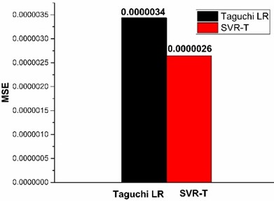
It is clear that the predictions of the $\epsilon$-SVR-T model align more closely with the experimental values compared to those predicted by the Taguchi LR. The $\epsilon$-SVR-T model demonstrates superior predictive performance compared to the Taguchi LR model. This is also evident from the performance metrics MSE, MAPE, and $R^2$ values, which have been calculated and shown in Table 5.

Table 5Table showing the computed performance metrics

	Taguchi LR	$\epsilon$-SVR-T
MSE	0.000003437	0.000002647
MAPE	2.13143147	1.684506892
$R^2$	0.997993552	0.998597607

The MSE for the predictions of the $\epsilon$-SVR-T model is 0.000002647, which is less than the MSE of the Taguchi LR model, whose value is 0.000003437. This is also depicted graphically as shown in Fig. 5.

Fig. 5Graphical representation of MSE of Taguchi LR and ε-SVR-T model

4.4. Developing a GUI for the $\mathit{\epsilon }$-SVR-T model

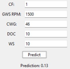
A GUI is modeled based on the ε-SVR-T model for the easy depiction of Ra predictions for settings as per the choice of the machinist. The picture of the GUI is shown in Fig. 6.

Fig. 6GUI based on the ε-SVR-T model

5. Observations

The following observations are drawn from this study.

1) It is found that the ML model ε-SVR is performing better for prediction than the remaining four ML models with MSE = 0.000088688, MAPE = 5.528787583, $R^2=$ 0.491078634.

2) The ε-SVR model is further refined by tuning its hyperparameters $C$, $\epsilon$, and the Kernel function using GridSearch CV. The best results are obtained when $C=$ 0.1, $\epsilon =$ 0.01, kernel = linear, and the testing results indicate the values of MSE = 0.000001638, MAPE = 0.988123699, $R^2=$0.988025649, showing considerable improvement in predictions by the model as compared to the other ML models and also with the Taguchi LR model proposed by the selected study.

3) The ε-SVR-T model is also tested with validation experiments of the selected study, the results of which show that the predicted outcomes of the suggested $\epsilon$-SVR-T model are better, with MSE = 0.000002647, MAPE = 1.684506892, $R^2=$ 0.998597607, as compared to the Taguchi LR model, which has MSE= 0.000003437, MAPE= 2.13143147, $R^2=$ 0.997993552.

6. Conclusions

The study undertook the predictive modeling of Ra obtained from the experimental study of the surface grinding using ML algorithms, namely LR, DT, RF, $\epsilon$-SVR, and KNN, and compared their performance. The $\epsilon$-SVR ML model outperformed the other four models in predictions. A GUI is modeled based on the $\epsilon$-SVR-T model for the easy predictions of Ra, which will help the machinist to have an early idea of the output response Ra before actually conducting the grinding process. The study also revealed that ML algorithms can be effectively used for developing the machining output response prediction models for important machining operations like surface grinding, and it could be extended to other machining operations as well.