Accurate vehicle state estimation using WOA-SVR algorithm: a novel approach

Cui, Dawei; Liu, Yingjie

doi:10.21595/jve.2025.25047

Journal of Vibroengineering

Browse Journal

Submit article

Published: 12 August 2025

Check for updates

Accurate vehicle state estimation using WOA-SVR algorithm: a novel approach

Dawei Cui¹

Yingjie Liu²

^{1, 2}School of Machinery and Automation, Weifang University, Weifang, 261061, Shandong, China

^{1, 2}Shandong Key Laboratory of Intelligent Manufacturing Technology for Advanced Power Equipment, Weifang, 261061, Shandong, China

Corresponding Author:

Yingjie Liu

Cite the article Download PDF

Article in Press

Downloads 24

Abstract

Accurate estimation of the state parameters of vehicles during driving has always been a focus of attention for researchers in the automotive industry. Traditional estimation methods have the problem of larger errors. For this issue, a motion state estimation algorithm based on whale optimization algorithm and support vector regression (WOA-SVR) that does not rely on accuracy of the vehicle model and vehicle parameters was proposed for estimating the yaw rate and side slip angle as well as longitudinal speed. Firstly, the dynamic characteristics of the vehicle were analyzed and a two-layer SVR estimation structure was constructed. Then, Carsim was used to collect data which was used to train SVR models on both sides of the estimation structure from various operating conditions. The WOA algorithm was used to optimize the penalty factor and kernel function parameter in the SVR algorithm to obtain the optimal algorithm parameters. Finally, the feasibility of the WOA-SVR algorithm was verified through Matlab/Simlink simulation and virtual experiments. The simulation results indicate that the root mean square error (RMSE) of the yaw rate and side slip angle as well as longitudinal speed improves 67.8 %, 63.5 %, 69.9 % respectively. The verification results indicate that the WOA-SVR algorithm has good estimation accuracy and robustness in vehicle state estimation.

Highlights

The simulation results indicate that the root mean square error(RMSE) of the yaw rate and side slip angle as well as longitudinal speed improves 67.8%, 63.5%, 69.9% respectively.
The proposed WOA-SVRV algorithm can solve the problem of vehicle state estimation with the performance of noise fluctuation suppression and higher estimation accuracy.
The verification results indicate that the WOA-SVR algorithm has good estimation accuracy and robustness in vehicle state estimation.

1. Introduction

With the development of the electrification and intelligence of automobiles, active control systems and intelligent driving assistance systems are gradually being applied. A reasonable approach is using low-cost sensors to obtain easily obtainable state information, such as longitudinal acceleration, lateral acceleration, wheel speed, etc., and then obtain parameters through estimation algorithms. Therefore, how to accurately and quickly obtain the driving states has become a hot research topic. The purpose is to determine the state variables during the vehicle driving process. It is not only a key technology for achieving active control of the vehicle chassis but also an important prerequisite for optimizing control in autonomous driving and human-machine co-driving problems. The longitudinal dynamics control of a vehicle includes: Traction Control System, Antilock Brake System. The lateral dynamics control of automobiles includes driving energy-saving control in autonomous driving and human-machine co-driving, and optimized control of trajectory following, all of which rely on accurate estimation of vehicle status. Some of these vehicle state variables cannot be directly measured and some of them require expensive sensor equipment and strict installation arrangements for measurement, and some measurement results require post-processing before they can be used, making many solutions unable to be installed on mass-produced vehicles due to cost issues and only suitable for configuration on research and development prototype vehicles. Therefore, mature and available vehicle state estimation schemes should be within an acceptable cost range, equipped with multiple direct or indirect measurement sensors, and achieve multi-source information fusion through vehicle state estimators to provide vehicle state data that meets the needs [1-3].

Ok et al. proposed a convolutional neural network estimator which could obtain the required variables without using expensive sensors [4-6]. Zhu et al. designed a Luenberger observer to provide data support for the active front wheel steering system in order to suppress internal and external interference [7]. Xing et al. constructed an adaptive particle filter by introducing the latest observation data, which had efficient estimation capability for nonlinear dynamic vehicle systems [8]. Liu et al. used EKF as a basis to reduce the impact of noise on estimation results by adjusting the noise covariance matrix in real-time [9]. Wan et al. designed an error minimization method for UKF under unknown noise conditions. By real-time correction of noise, the robustness of the algorithm was improved [10]. Xia et al. established a cubature Kalman filter (CKF) method and verified the effectiveness of the estimation algorithm through real vehicle experiments [11]. The above-mentioned research objects were mostly traditional automobiles, and the Kalman filter estimation algorithm was based on the improvement of the algorithm on the basis of third-order accuracy, which limited its accuracy improvement. Other estimation algorithms mainly fused different algorithms, which were computationally complex and had high constraint levels on the algorithm. They did not have high estimation accuracy for high-dimensional nonlinear models. It can not only handle simple linear systems, but also complex multidimensional nonlinear systems [12-14]. Liu et al. proposed a limited memory filter (LMF) that stores historical measurement data of a certain memory length, calculates the conditional probability density function and its parameters, namely the mean and covariance matrix, under nonlinear conditions overcoming the divergence of the filter [15]. Liu et al. proposed an extended Kalman algorithm with limited memory noise online estimation to address the statistical lag problem of gradient noise in new residual sequences, which improved the filtering detection speed and computational accuracy to a certain extent [16]. Lv et al. combined the minimum model error criterion with EK filtering to propose a state estimation system that considered arbitrary nonlinear model errors and Gaussian white noise. This system could effectively detect dynamic errors and use them for model updating [17]. Park proposed a new adaptive random weighting filtering algorithm and established a random weighting theory under limited memory conditions [18]. Simulation analysis indicated that this algorithm could effectively suppress the influence of unknown statistical characteristics of measurement noise.

Therefore, this article proposes a vehicle motion state estimation algorithm based on WOA-SVR. By analyzing the basic dynamic characteristics of the vehicle itself, an SVR algorithm structure is designed to achieve the estimation of the vehicle motion state. Then, Carsim/Simulink is used to collect data from various operating conditions and train the SVR model. During the model training process, the WOA algorithm is used to optimize the penalty factor and kernel function parameter in the SVR relaxation variables. Finally, the feasibility of the WOA-SVR algorithm is verified through simulation and virtual experiment.

2. Mathematical model of vehicle state estimation problem

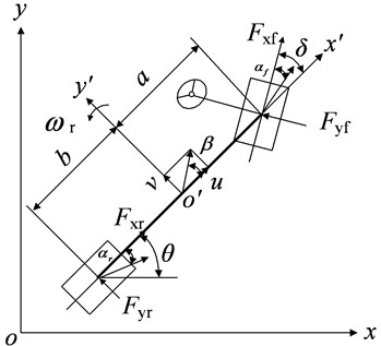
2.1. 3-DOF vehicle model

It is assumed that the influence of the steering transmission mechanism on the two front wheel steering angles is ignored; The vehicle is in planar motion; The pitch and roll motion and their coupling as well as the influence of suspension are ignored; The bouncing between the body and chassis is ignored; The influence of wheel camber angle and return torque on the vehicle dynamic performance is ignored. The vehicle state estimation model is established based on a 3-DOF vehicle model.

The dynamic equation of the 3-DOF vehicle model is as follows Eqs. (1-4) [19]:

1

{\dot{ω}}_{r} = \frac{a^{2} k_{1} + b^{2} k_{2}}{I_{z}} \frac{ω_{r}}{u} + \frac{a k_{1} - b k_{2}}{I_{z}} β - \frac{a k_{1}}{I_{z}} δ,

2

\dot{β} = \frac{a k_{1} - b k_{2} - m u^{2}}{m} \frac{ω_{r}}{u^{2}} + \frac{k_{1} + k_{2}}{m} \frac{β}{u} - \frac{k_{1} δ}{m u},

3

\dot{u} = a_{x} + v x,

4

a_{y} = \frac{a k_{1} - b k_{2}}{m u} ω_{r} + \frac{k_{1} + k_{2}}{m} β - \frac{k_{1}}{m} δ .

The side slip angle of the center of mass is:

5

β = \arctan (\frac{v}{u}) .

2.2. Tire model

The brush tire model and the magic formula tire model can accurately describe the nonlinear relationship between the longitudinal and lateral forces of the tire and the side slip angle, slip ratio, tire vertical load, and road adhesion coefficient. Under normal driving conditions of a vehicle, when the tire side slip angle is small, the lateral force of the tire is linearly related to the side slip angle, and the lateral force of the tire can be linearized as [19]:

6

\{\begin{matrix} F_{y f} = c_{f} α_{f}, \\ F_{y r} = c_{r} α_{r}, \end{matrix}

where $c_{f}$ and $c_{r}$ are the lateral stiffness values of the front and rear tires. $α_{f}$ and $α_{r}$ are the front and rear slip angles:

7

ξ^{d o w n} = (ξ_{1}^{d o w n}, ξ_{2}^{d o w n}, \dots, ξ_{m}^{d o w n}) .

Fig. 13-DOF vehicle model

3. WOA-SVR method

3.1. Support vector regression (SVR) algorithm

If there are $m$ circular dots distributed in a two-dimensional plane, then the given dataset $T$ is [20-21]:

8

T = \{(x^{(1)}, y^{(1)}), (x^{(2)}, y^{(2)}), \dots, (x^{(m)}, y^{(m)},)\} .

The sample points in dataset $T$ are fitted onto hyperplane $h (x^{(i)}) = φ (x^{(i)}) θ^{(i)} + b$ , where $φ (x^{(i)})$ is the data point on the plane; $θ = (θ^{(1)}, θ^{(2)}, \dots, θ^{(i)})$ is the model parameter vector; $b$ is the bias. The sample points farthest from the hyperplane are called support vectors. The geometric interval $d$ between the support vectors and the hyperplane $h (x^{(i)})$ is:

9

d = y^{(i)} \cdot (φ (x^{(i)}) θ^{(i)} + b) \cdot \frac{1}{‖θ‖} .

It is assumed that there are $n$ support vectors. The relaxation variables are added to maximize the interval. And the objective function becomes:

10

\underset{θ, b, ξ^{u p}, ξ^{d o w n}}{m i n} \frac{1}{2} {‖θ‖}_{2}^{2} + c \sum_{i = 1}^{m} (ξ_{i}^{u p} + ξ_{i}^{d o w n}),

s . t . \{\begin{array}{l} y^{(i)} - φ (x^{(i)}) θ^{(i)} - b \leq ξ_{i}^{u p} + ε, \\ \begin{matrix} φ (x^{(i)}) θ^{(i)} + b - y^{(i)} \leq ξ_{i}^{d o w n} + ε, \\ ξ_{i}^{u p} \geq 0, ξ_{i}^{d o w n} \geq 0, \end{matrix} \end{array}

where $ξ^{u p}$ and $ξ^{d o w n}$ are the up and low bound vectors of the relaxation variables; $ξ^{u p} = (ξ_{1}^{u p}, ξ_{2}^{u p}, \dots, ξ_{m}^{u p})$ ; $ξ^{d o w n} = (ξ_{1}^{d o w n}, ξ_{2}^{d o w n}, \dots, ξ_{m}^{d o w n})$ ; $c$ is the penalty coefficient; $ε$ is the tolerance of losses.

The penalty coefficient $c c > 0$ is used to control the balance between the interval and the relaxation variable penalties. Then the quadratic programming problem is transformed into a convex optimization problem. The Lagrange function is constructed as follows:

11

L (θ^{(i)}, b, ξ_{i}^{u p}, ξ_{i}^{d o w n}, λ_{i}^{u p}, λ_{i}^{d o w n}, μ_{i}^{u p}, μ_{i}^{d o w n})

= \frac{1}{2} {‖θ‖}_{2}^{2} + c \sum_{i = 1}^{m} (ξ_{i}^{u p} + ξ_{i}^{d o w n}) + \sum_{i = 1}^{n} μ_{i}^{u p} ξ_{i}^{u p} - \sum_{i = 1}^{n} μ_{i}^{d o w n} ξ_{i}^{d o w n} + \sum_{i = 1}^{n} λ_{i}^{u p} [y^{(i)} - φ (x^{(i)}) θ^{(i)} - b - ξ_{i}^{u p} - ε)] + \sum_{i = 1}^{n} λ_{i}^{d o w n} [φ (x^{(i)}) θ^{(i)} + b - y^{(i)} - ξ_{i}^{d o w n} - ε)],

where $λ_{i}^{u p}$ , $λ_{i}^{d o w n}$ , $μ_{i}^{u p}$ , $μ_{i}^{d o w n}$ are the Lagrange variables.

The results of each parameter can be obtained by taking partial derivatives of parameter $θ^{(i)}$ , $b$ , $ξ_{i}^{u p}$ , $ξ_{i}^{d o w n}$ and making each partial derivative equal to 0. Eq. (12) can be obtained by inputting the results of each parameter into Eq. (11):

12

L (θ^{(i)}, b, ξ_{i}^{u p}, ξ_{i}^{d o w n}, λ_{i}^{u p}, λ_{i}^{d o w n}, μ_{i}^{u p}, μ_{i}^{d o w n})

= \frac{1}{2} θ^{T} θ + c \sum_{i = 1}^{n} ξ_{i}^{u p} - \sum_{i = 1}^{n} μ_{i}^{u p} ξ_{i}^{u p} - \sum_{i = 1}^{n} λ_{i}^{u p} φ (x^{(i)}) θ^{(i)} + \sum_{i = 1}^{n} λ_{i}^{u p} b + \sum_{i = 1}^{n} λ_{i}^{u p} y^{(i)} - \sum_{i = 1}^{n} λ_{i}^{u p} ξ_{i}^{u p} - \sum_{i = 1}^{n} λ_{i}^{u p} ε + c \sum_{i = 1}^{n} ξ_{i}^{d o w n} - \sum_{i = 1}^{n} μ_{i}^{d o w n} ξ_{i}^{d o w n} + \sum_{i = 1}^{n} λ_{i}^{d o w n} φ (x^{(i)}) θ^{(i)} + \sum_{i = 1}^{n} λ_{i}^{d o w n} b - \sum_{i = 1}^{n} λ_{i}^{d o w n} y^{(i)} - \sum_{i = 1}^{n} λ_{i}^{d o w n} ξ_{i}^{d o w n} - \sum_{i = 1}^{n} λ_{i}^{d o w n} ε = \sum_{i = 1}^{n} y^{(i)} (λ_{i}^{u p} - λ_{i}^{d o w n}) - ε \sum_{i = 1}^{n} (λ_{i}^{u p} + λ_{i}^{d o w n})

- \frac{1}{2} \sum_{i = 1}^{n} (λ_{i}^{u p} - λ_{i}^{d o w n}) φ (x) \sum_{i = 1}^{n} (λ_{j}^{u p} - λ_{j}^{d o w n}) (φ (x))^{T} = \sum_{i = 1}^{n} [y^{(i)} (λ_{i}^{u p} - λ_{i}^{d o w n}) - ε (λ_{i}^{u p} + λ_{i}^{d o w n})] - \frac{1}{2} \sum_{i = 1}^{n} \sum_{j = 1}^{n} (λ_{i}^{u p} - λ_{i}^{d o w n}) (λ_{j}^{u p} - λ_{j}^{d o w n}) φ (x) (φ (x))^{T} .

By minimizing the value of $ξ_{i}^{u p}$ , $ξ_{i}^{d o w n}$ corresponding to Eq. (12), the optimal value of the model parameter $θ$ can be derived:

13

θ^{*} = \sum_{i = 1}^{n} (λ_{i}^{u p} - λ_{i}^{d o w n}) {[φ (x)]}^{T} .

The KKT condition for SVR is:

14

\{\begin{matrix} λ_{i}^{u p} (y^{(i)} - φ (x^{(i)}) θ^{(i)} - b - ξ_{i}^{u p} - ε) = 0, \\ λ_{i}^{d o w n} (φ (x^{(i)}) θ^{(i)} + b - y^{(i)} - ξ_{i}^{d o w n} - ε) = 0, \\ y^{(i)} - φ (x^{(i)}) θ^{(i)} - b - ξ_{i}^{u p} - ε \leq 0, \\ φ (x^{(i)}) θ^{(i)} + b - y^{(i)} - ξ_{i}^{d o w n} - ε \leq 0, \\ (c - λ_{i}^{d o w n}) ξ_{i}^{d o w n} = 0, (c - λ_{i}^{d o w n}) ξ_{i}^{d o w n} = 0, \\ ξ_{i}^{u p} ξ_{i}^{d o w n} = 0, ξ_{i}^{u p} \geq 0, ξ_{i}^{d o w n} \geq 0, \\ 0 \leq λ_{i}^{u p}, λ_{i}^{d o w n} \leq c, u p_{i} λ_{i}^{d o w n} = 0 . \end{matrix}

According to the KKT condition of SVR, multiple $b^{(i)}$ can be obtained by $b^{(i)} = y^{(i)} - φ (x^{(i)}) θ^{i} - ε$ , and the average of multiple $b^{(i)}$ values can be used as the final result:

15

b^{*} = \frac{1}{n} \sum_{i = 1}^{n} b^{(i)} .

The final SVR hyperplane can be obtained by substituting $θ^{*}$ and $b^{*}$ into the hyperplane expression:

16

{\hat{y}}^{(i)} = φ (x^{(i)}) θ^{* (i)} + b^{*} = \sum_{i = 1}^{n} (λ_{i}^{u p} - λ_{i}^{d o w n}) φ (x) (φ (x))^{T} - \frac{1}{n} \sum_{i = 1}^{n} (y^{(i)} + ε) - \frac{1}{n} \sum_{i = 1}^{n} [\sum_{j = 1}^{n} (λ_{i, j}^{u p} - λ_{i, j}^{d o w n})] φ (x) (φ (x))^{T} .

3.2. Selection of kernel function

When the dataset is not linearly separable in the original features, a kernel function $Φ (\cdot)$ is introduced in the support vector machine, and then performing dataset classification in the high-dimensional space. The kernel function is used to solve the calculation of sample distance $‖Φ (x_{i}) - Φ (x_{j})‖$ after mapping which is expressed as:

17

{‖Φ (x_{i}) - Φ (x_{j})‖}^{2} = k (x_{i}, x_{i}) - 2 k (x_{i}, x_{j}) + k (x_{j}, x_{j}) .

The commonly used Gaussian kernel function is:

18

k (x_{i}, x_{j}) = \exp (- \frac{{‖x_{i} - x_{j}‖}^{2}}{2 g^{2}}),

where $g$ is the kernel function parameter.

3.3. WOA optimization algorithm

The distance and position vector between individuals in the WOA algorithm are [22]:

19

\{\begin{matrix} D = |C \cdot X^{*} (t) - X (t)|, \\ X (t + 1) = X^{*} (t) - A \cdot D, \end{matrix}

where $t$ is the current iteration count; $D$ is the distance vector between the current whale and the random whale; $X (t)$ is the position vector; $X^{*} (t)$ is the position vector of the currently obtained best solution; $A$ and $C$ are the coefficients, $A = 2 a (t) r_{1} (t)$ , $C = 2 r_{2} (t)$ . During the entire iteration process, the convergence factor $a$ linearly decreases from 2 to 0; $r_{1}$ and $r_{2}$ are random vectors in [0, 1].

Fig. 2Processing of WOA optimizing the SVR parameters

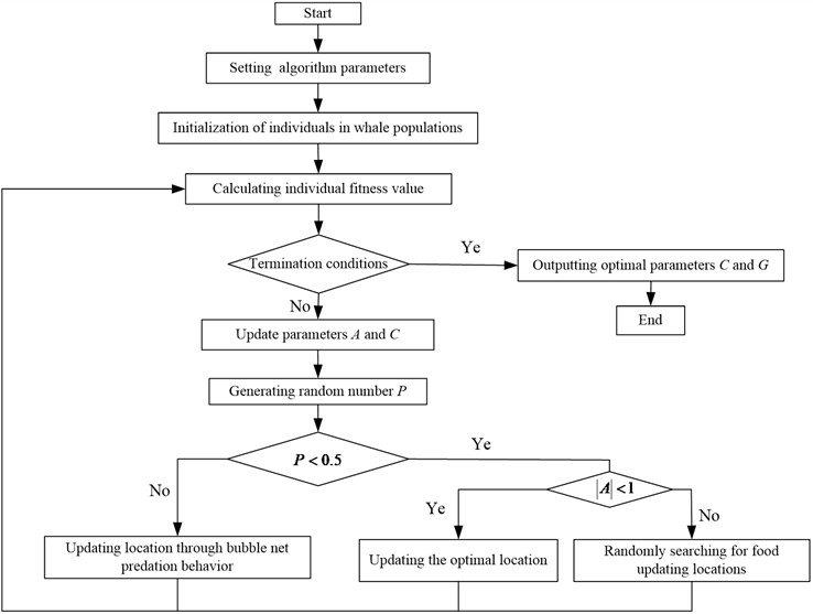
There are two main mechanisms for whale predation in the WOA algorithm: encirclement predation and bubble net predation. The position updating formula is as follows:

20

X (t + 1) = \{\begin{array}{l} X^{*} (t) - A D, p \leq 0.5, \\ D^{'} \exp (B L) \cos (2 π L) + X^{*} (t), p > 0.5 . \end{array}

When $|A| \geq 1$ , the search individual will swim towards the random whale to obtain the optimal solution:

21

\{\begin{matrix} D^{''} = C \cdot X_{r a n d} (t) - X (t), \\ X (t + 1) = X_{r a n d} (t) - A \cdot D, \end{matrix}

where $D^{''}$ is the distance vector between the current search individual and the random individual; $X_{r a n d} (t)$ is the current position of the random individual.

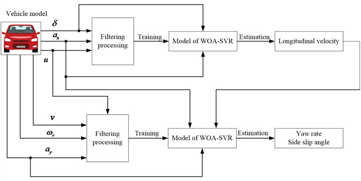
The processing of WOA optimizing the SVR parameters is shown in Fig. 2. And the structure diagram of WOA-SVR state estimation is shown in Fig. 3.

Fig. 3Structure diagram of WOA-SVR state estimation

4. Numerical simulation and experimental verification

4.1. Numerical simulation

To verify the performance of the proposed algorithm, a certain type of vehicle is verified by a simulation test in the CarSim software.

CarSim is a simulation software developed by the American company Mechanical Simulation specifically for vehicle dynamics. Used by over 30 automobile manufacturers, 60 automobile parts manufacturers, and more than 160 research institutions and universities worldwide, it has quickly become a leader in the field of vehicle dynamics simulation software since its inception. Due to its ability to realistically reproduce the response of vehicles to external inputs such as drivers, road surfaces, and aerodynamics through 3D animation, CarSim has been widely used in simulation tests of vehicle comfort, braking performance, and handling stability. Research has shown that the algorithm of the Carsim has good predictive performance for vehicle dynamics and different operating conditions, and has high reliability. CarSim software provides three different ways of solvers for researchers to use, namely CarSim internal model solver, custom model solver extended through C language interface, and custom model solver extended through MATLAB/Simulink. Through the latter two solvers, users can easily expand the internal models of CarSim and integrate user-defined models into vehicle model for dynamics simulation to verify the accuracy of the user-defined models.

To verify the estimation accuracy of the WOA-SVR algorithm, the CKF is used as the comparison object in this paper. The steering wheel angle is the input. The vehicle parameters in the Carsim are as follows: $I_{z} =$ 2765 kg·m²; $m =$ 1845 kg; $a =$ 1.40 m; $b =$ 1.55 m.

Fig. 4Flow chart of co-simulation of Carsim and Matlab/Simulink

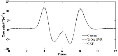
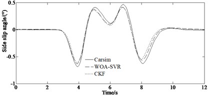
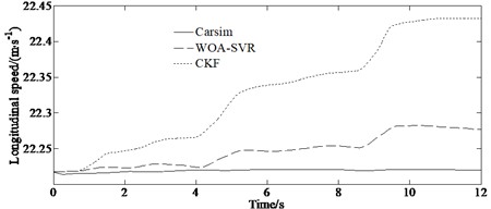
4.1.1. Double lane changing condition

The double lane changing condition is used in the simulation experiment with a speed of 80 km/h and a road adhesion coefficient of 0.85.

Fig. 5 is the simulation results under the double lane changing condition. It can be seen from Figs. 5(a)-(b) that the estimated values of the CKF and the WOA-SVR algorithms are closer to the reference values. And also, both algorithms have different degrees of divergence, and the reason for this may be that the tires enter the nonlinear area when the vehicle is cornering at high speed. The comparison between the constructed prediction method and other estimation method shows that the WOA-SVR algorithm proposed in this paper is effective, feasible, and has higher accuracy. Fig. 5(c) indicates that the proposed method has smaller errors compared to other algorithm, indicating that it has good generalization ability and can achieve good vehicle motion state prediction results, and has high practical value. This is because the estimation results are optimized iteratively by utilizing the performance of the fast convergence and easy escape from local optima of whale optimization algorithm obtaining the optimized results through simulation. However, the computational cost of the algorithm is relatively high, and further optimization is needed in practical applications.

Fig. 5Simulation results: a) yaw rate, b) side slip angle, c) longitudinal speed

a)

b)

c)

The computation cost is shown in Tables 1. From Tables 1 it can be seen that the WOA-SVR algorithm does not have too high computation cost. We can adopt an elite retention strategy by only conducting fine searches in the vicinity of the current optimal solution to reduce the computational complexity of global searches.

Table 1Comparison of the computation cost under the double lane changing condition

Algorithms	Total times (s)
CKF	6.317
WOA-SVR	6.382

4.1.2. Serpentine condition

The serpentine condition is used in the simulation experiment with a speed of 65 km/h and a road adhesion coefficient of 0.85.

Fig. 6 is the simulation result under the serpentine condition. It can be seen from Figs. 6(a)-(b) that the estimated values of the WOA-SVR algorithm are closer to the actual values. And the estimation accuracy of the WOA-SVR algorithm is always better than that of the CKF. Fig. 6(c) indicates that the proposed method has smaller errors compared to other algorithm. This is because the SVR is a machine learning method suitable for small sample and multi-dimensional data. Compared to traditional estimation method, the SVR method has better performance in estimation, good non-linear regression and generalization abilities, faster training speed. And the SVR model performs well in small sample situations with strong generalization ability. It has a large number of kernel functions to use and can flexibly solve regression problems.

Fig. 6Simulation results: a) yaw rate, b) side slip angle, c) longitudinal speed

a)

b)

c)

The root mean square error (RMSE) and average absolute error (MAE)of the estimation value relative to the virtual test value are given to verify the accuracy of the proposed algorithm which are shown in Table 1.

Table 2 indicates that the WOA-SVR algorithm has significant advantages compared to the traditional CKF algorithm under simulation verification conditions. The RMSE and MAE values of traditional CKF is significantly higher than that of WOA-SVR algorithm demonstrating that the WOA-SVR has a smaller estimation error and higher estimation accuracy.

4.2. Experimental verification

The Carsim software is used for a virtual vehicle test to verify the effectiveness of the proposed algorithm.

Table 2RMSE and MAE indicators under the double lane changing condition

Evaluation index	State value	CKF	WOA-SVR
RMSE	$ω_{r}$ (deg/s)	0.9638	0.3102
	$β$ (deg)	0.1868	0.0682
	$u$ (km/h)	0.8463	0.2539
MAE	$ω_{r}$ (deg/s)	0.0165	0.0142
	$β$ (deg)	0.0022	0.0019
	$u$ (km/h)	0.6363	0.1911

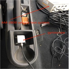
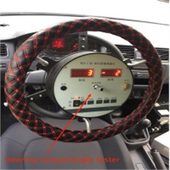
At the same time, a real vehicle test is conducted to verify the effectiveness of the algorithm. The real experiment vehicle and the measurement equipment’s are shown in Fig. 7 and Fig. 8 respectively.

Fig. 7Real test vehicle

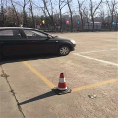
Fig. 8Measurement equipments

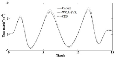
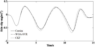
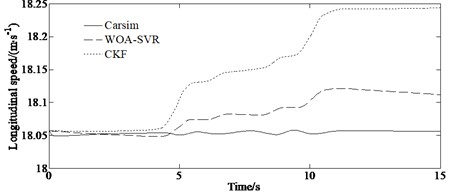
From Figs. 9(a)-(b) it can be seen that the WOA-SVR algorithm does not produce large errors due to the sudden changes in the steering wheel while the CKF method has a large deviation compared with the value from the actual vehicle experiment. This is because that by using the WOA algorithm for optimizing the penalty function and kernel function parameters of SVR, the algorithm is simple and can quickly escape the local optimal trap during training, with fast convergence speed. The WOA-SVR method can be applied to estimate vehicle motion state obtaining good estimation results with high accuracy and reliability as well as precision. Fig. 9(c) shows the CKF algorithm generates a larger divergence after 5 s. This indicates that the WOA-SVR algorithm has high robustness and accuracy.

5. Conclusions

This article proposes a vehicle motion state estimation algorithm based on WOA-SVR. By analyzing the basic dynamic characteristics of the vehicle itself, an SVR algorithm structure is designed to achieve machine learning estimation of the vehicle motion state. Then the Carsim software is used to collect data from various driving conditions and train the SVR model. During the model training process, the WOA method is used to optimize the penalty factor and kernel function parameter in the SVR relaxation variables. Finally, the feasibility of using the WOA-SVR algorithm to estimate the vehicle state is verified through MATLAB simulation and virtual vehicle experiments. The verification results show that the WOA-SVR algorithm has good estimation accuracy and robustness to changes in vehicle speed, and can achieve accurate estimation of vehicle motion states without relying on dynamic models.

Fig. 9Comparison of estimated and test values: a) yaw rate, b) side slip angle, c) longitudinal speed

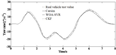
a)

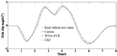
b)

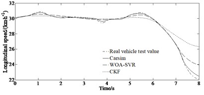
c)

In the future, the factors of affecting the sensitivity, convergence speed, and convergence accuracy of control parameters can be analyzed theoretically. And how to effectively balance the local development ability and global exploration ability of algorithms should be researched to provide theoretical support for the practical application of WOA-SVR. At the same time, how to further improve the algorithm's efficiency is the future research direction.

References

Y. Liu, D. Cui, and W. Peng, “Optimum control for path tracking problem of vehicle handling inverse dynamics,” Sensors, Vol. 23, No. 15, p. 6673, Jul. 2023, https://doi.org/10.3390/s23156673

Publisher
Y. Liu, D. Cui, and W. Peng, “optimal lane changing problem of vehicle handling inverse dynamics based on mesh refinement method,” IEEE Access, Vol. 11, pp. 115617–115626, Jan. 2023, https://doi.org/10.1109/access.2023.3324422

Publisher
Y. Liu and D. Cui, “Vehicle dynamics prediction via adaptive robust unscented particle filter,” Advances in Mechanical Engineering, Vol. 15, No. 5, p. 168781322311707, May 2023, https://doi.org/10.1177/16878132231170766

Publisher
M. Ok, S. Ok, and J. H. Park, “Estimation of vehicle attitude, acceleration, and angular velocity using convolutional neural network and dual extended Kalman filter,” Sensors, Vol. 21, No. 4, p. 1282, Feb. 2021, https://doi.org/10.3390/s21041282

Publisher
H. Ikhlef, S. Bourebia, and A. Melit, “Link state estimator for VANETs using neural networks,” Journal of Network and Systems Management, Vol. 32, No. 1, pp. 3–15, Nov. 2023, https://doi.org/10.1007/s10922-023-09786-5

Publisher
G. Yi, X. Zhuang, and Y. Li, “Probabilistic state estimation in district heating grids using deep neural network,” Sustainable Energy, Grids and Networks, Vol. 38, p. 101353, Jun. 2024, https://doi.org/10.1016/j.segan.2024.101353

Publisher
Y. Zhu and L. Ma, “Composite chattering-free discrete-time sliding mode controller design for active front steering system of electric vehicles,” Nonlinear Dynamics, Vol. 105, No. 1, pp. 301–313, Jun. 2021, https://doi.org/10.1007/s11071-021-06465-5

Publisher
D. X. Xing et al., “Vehicle state estimation based on adaptive cubature particle filtering,” (in Chinese), Journal of Nanjing University of Aeronautics and Astronautics, Vol. 52, No. 3, pp. 445–453, 2020, https://doi.org/10.16356/j.1005-2615.2020.03.013

Publisher
M. C. Liu, Z. B. Peng, and X. J. Wu, “Joint estimation of vehicle motion state based on adaptive fuzzy extended Kalman filter,” (in Chinese), Automobile Technology, Vol. 4, pp. 23–30, 2022, https://doi.org/10.19620/j.cnki.1000-3703.20210263

Publisher
W. Wan, J. Feng, B. Song, and X. Li, “Huber-based robust unscented Kalman filter distributed drive electric vehicle state observation,” Energies, Vol. 14, No. 3, p. 750, Feb. 2021, https://doi.org/10.3390/en14030750

Publisher
G. Reina and A. Messina, “Vehicle dynamics estimation via augmented Extended Kalman Filtering,” Measurement, Vol. 133, pp. 383–395, Feb. 2019, https://doi.org/10.1016/j.measurement.2018.10.030

Publisher
Y. Wang et al., “Tire tateral forces and sideslip angle estimation for distributed drive electric vehicle using noise adaptive cubature Kalman filter,” (in Chinese), Journal of Mechanical Engineering, Vol. 55, No. 22, p. 103, Jan. 2019, https://doi.org/10.3901/jme.2019.22.103

Publisher
A. Alshawi et al., “An adaptive unscented Kalman filter for the estimation of the vehicle velocity components, slip angles, and slip ratios in extreme driving manoeuvres,” Sensors, Vol. 24, No. 2, p. 436, Jan. 2024, https://doi.org/10.3390/s24020436

Publisher
A. Jazwinski, “Limited memory optimal filtering,” IEEE Transactions on Automatic Control, Vol. 13, No. 5, pp. 558–563, Oct. 1968, https://doi.org/10.1109/tac.1968.1098981

Publisher
X. X. Liu, X. S. Xu, and A. G. Feng, “Improved algorithm for limited memory on-line estimating Kalman filter,” Joural of Southeast University (Natural Science Edition), Vol. 40, No. 4, pp. 766–770, 2010, https://doi.org/10.3969/j.issn.1001-0505.2010.04.020

Publisher
W. Liu, H. He, and F. Sun, “Vehicle state estimation based on minimum model error criterion combining with extended Kalman filter,” Journal of the Franklin Institute, Vol. 353, No. 4, pp. 834–856, Mar. 2016, https://doi.org/10.1016/j.jfranklin.2016.01.005

Publisher
D. Lv, Z. Gao, D. Mu, Y. Zhong, and C. Gu, “Limited memory measurement noise adaptive random weighted filtering algorithm,” in IEEE 8th International Conference on Computer Science and Network Technology (ICCSNT), pp. 127–132, Nov. 2020, https://doi.org/10.1109/iccsnt50940.2020.9305017

Publisher
G. Park, “Optimal vehicle position estimation using adaptive unscented Kalman filter based on sensor fusion,” Mechatronics, Vol. 99, p. 103144, May 2024, https://doi.org/10.1016/j.mechatronics.2024.103144

Publisher
Y. Liu, D. Cui, and W. Peng, “Vehicle state and parameter estimation based on improved extend Kalman filter,” Journal of Measurements in Engineering, Vol. 11, No. 4, pp. 496–508, Dec. 2023, https://doi.org/10.21595/jme.2023.23475

Publisher
N. Guo and Z. Wang, “A combined model based on sparrow search optimized BP neural network and Markov chain for precipitation prediction in Zhengzhou City, China,” Journal of Water Supply: Research and Technology-Aqua, Vol. 71, No. 6, pp. 782–800, Jun. 2022, https://doi.org/10.2166/aqua.2022.047

Publisher
Y. You et al., “Vehicle motion state estimation based on WOA-SVR,” (in Chinese), China Mechanical Engineering, Vol. 35, No. 6, pp. 973–981, 2024, https://doi.org/10.3969/j.issn.1004-132x.2024.06.003

Publisher
Q. Guo, B. Qiao, Y. Yang, and J. Guo, “Research on parameter inversion of coal mining subsidence prediction model based on improved whale optimization algorithm,” Energies, Vol. 17, No. 5, p. 1158, Feb. 2024, https://doi.org/10.3390/en17051158

Publisher

About this article

Received

07 May 2025

Accepted

04 July 2025

Published

12 August 2025

SUBJECTS

Vibration in transportation engineering

DOI

https://doi.org/10.21595/jve.2025.25047

Keywords

vehicle dynamics

vehicle state estimation

whale optimization algorithm

support vector regression

Acknowledgements

This research was supported by the Open Research Program of Huzhou Key Laboratory of Urban Multidimensional Perception and Intelligent Computing under Grant No. UMPIC202404.

Data Availability

The datasets generated during and/or analyzed during the current study are available from the corresponding author on reasonable request.

Author Contributions

Dawei Cui: mathematical model and simulation techniques. Yingjie Liu: spelling and grammar checking as well as software.

Conflict of interest

The authors declare that they have no conflict of interest.

This is an open access article distributed under the Creative Commons Attribution License, which permits unrestricted use, distribution, and reproduction in any medium, provided the original work is properly cited.

D. Cui and Y. Liu, “Accurate vehicle state estimation using WOA-SVR algorithm: a novel approach,” Journal of Vibroengineering, Vol. 27, No. 6, –12, Aug. 2025, https://doi.org/10.21595/jve.2025.25047

Copy Extrica

Copied to clipboard!

TY  - JOUR
DO  - 10.21595/jve.2025.25047
UR  - https://doi.org/10.21595/jve.2025.25047
TI  - Accurate vehicle state estimation using WOA-SVR algorithm: a novel approach
T2  - Journal of Vibroengineering
AU  - Cui, Dawei
AU  - Liu, Yingjie
PY  - 2025
DA  - 2025/08/12
PB  - Extrica
VL  - 27
IS  - 6
SN  - 1392-8716
SN  - 2538-8460
ER  - 

Copy Ris

Copied to clipboard!

 @article{Cui_2025, title={Accurate vehicle state estimation using WOA-SVR algorithm: a novel approach}, ISSN={2538-8460}, url={https://doi.org/10.21595/jve.2025.25047}, DOI={10.21595/jve.2025.25047}, journal={Journal of Vibroengineering}, publisher={JVE International Ltd.}, author={Cui, Dawei and Liu, Yingjie}, year={2025}, month=aug }

Copy Bibtex

Copied to clipboard!

[1]D. Cui and Y. Liu, “Accurate vehicle state estimation using WOA-SVR algorithm: a novel approach,” Journal of Vibroengineering, Aug. 2025, doi: 10.21595/jve.2025.25047.

Copy IEEE

Copied to clipboard!

Cui, Dawei, and Yingjie Liu. “Accurate Vehicle State Estimation Using WOA-SVR Algorithm: A Novel Approach.” Journal of Vibroengineering, August 12, 2025. https://doi.org/10.21595/jve.2025.25047.

Copy Chicago

Copied to clipboard!

Accurate vehicle state estimation using WOA-SVR algorithm: a novel approach

Abstract

Highlights

1. Introduction

2. Mathematical model of vehicle state estimation problem

2.1. 3-DOF vehicle model

2.2. Tire model

3. WOA-SVR method

3.1. Support vector regression (SVR) algorithm

3.2. Selection of kernel function

3.3. WOA optimization algorithm

4. Numerical simulation and experimental verification

4.1. Numerical simulation

4.1.1. Double lane changing condition

4.1.2. Serpentine condition

4.2. Experimental verification

5. Conclusions

References

About this article

Related Articles