Measurement and estimation of vehicle state based on improved maximum correntropy square-root cubature Kalman filter

Liu, Yingjie; Cui, Dawei; Xie, Chenglian

doi:10.21595/jme.2025.24792

Journal of Measurements in Engineering

Browse Journal

Submit article

Published: 01 June 2025

Check for updates

Measurement and estimation of vehicle state based on improved maximum correntropy square-root cubature Kalman filter

Yingjie Liu¹

Dawei Cui²

Chenglian Xie³

¹Huzhou Key Laboratory of Urban Multidimensional Perception and Intelligent Computing, Huzhou 313000, P. R. China

^{1, 2}School of Machinery and Automation, Weifang University, Weifang 261061, Shandong, China

³Shandong Industrial Technician College, Weifang 261053, Shandong, China

Corresponding Author:

Yingjie Liu

Cite the article Download PDF

Article in Press

Downloads 164

Abstract

The acquisition of vehicle driving state parameters is the foundation for the active safety of vehicles. However, due to the cost or parameters of sensors that cannot be directly measured, accurate estimation of vehicle driving state parameters by low-cost estimators is crucial. In order to solve this problem, a 3-DOF nonlinear vehicle dynamic model was established firstly. Secondly, based on the principle of iterative maximum correntropy criterion (IMCC), the filtering error was reduced by optimizing the minimum noise covariance matrix to ensure the convergence and stability of long-term filtering. Combined with the adaptive iterative cubature Kalman filter (AICKF) algorithm, the process and measurement of noise covariance were updated to improve the accuracy and robustness of the estimation. Finally, the Carsim and Matlab/Simulink simulation platforms were combined, and simulation experiments were conducted under two different operating conditions, which were verified through real vehicle experiments. The results indicate that compared to the cubature Kalman Filter (CKF) algorithm, the algorithm of iterative maximum correntropy criterion of adaptive iterative cubature Kalman filter (IMCC-AICKF) has higher estimation accuracy for yaw rate and side slip angle as well as longitudinal velocity.

Highlights

The IMCC-AICKF algorithm can adapt to complex working conditions and has better accuracy in vehicle state estimation than traditional state estimation algorithms.
The proposed IMCC-AICKF algorithm can solve the problem of vehicle state estimation with the performance of noise fluctuation suppression and higher estimation accuracy.
The IMCC-AICKF has higher estimation accuracy for yaw rate and side slip angle as well as longitudinal velocity.

1. Introduction

The increasing number of vehicles in various countries around the world not only makes people’s life more comfortable, but also increases the risk of traffic accidents. In order to reduce the incidence and death toll of traffic accidents, an active safety technology for automobiles has flourished since the 1990s. At present, the current estimation methods presume the application of a model to estimate the vehicle driving status. And model parameters have a significant impact on the estimation results. Fixed values are often used to estimate model parameters. The estimation algorithm is mainly based on Kalman filtering and unscented Kalman filtering theory. Cubature Kalman filtering (CKF) theory has been applied in driving state estimation due to its ability to effectively solve nonlinear and divergence problems [1-3].

At present, the Kalman filter algorithm is widely used to design observers for estimating state parameters such as vehicle speed [4]. In recent years, the improved Kalman filter algorithm has been widely used in the state estimation for four-wheel motor vehicles. The extended Kalman filter (EKF) theory can achieve state estimation of nonlinear systems in the entire vehicle, but this method requires the calculation of complex Jacobian matrices and is affected by linearization errors. Unscented Kalman filter (UKF) has been well applied in state estimation of four-wheel drive vehicles. However, its accuracy in estimating vehicle parameters will significantly decrease under strong nonlinear system conditions [5-7]. The idea of particle filter (PF) is to use a set of particles to represent probabilities and to extract random state particles from posterior probabilities to express their distributions. However, this method may result in a loss of sample validity and diversity during the resampling stage, leading to sample impoverishment. Many scholars used particle swarm optimization particle filtering algorithm to achieve the vehicle state estimation, leading to proper results. The Unscented Particle Filter (UPF) algorithm ensures good consistency between the prior probability peak and the likelihood function peak, thereby reducing the particle degradation. However, its computational accuracy is affected by system noise uncertainty and lacks an adaptive adjustment mechanism [8-10].

Chen et al. used the cubature Kalman Filter (CKF) algorithm to calculate the posterior probability density, and was currently the closest algorithm to the Bayesian filtering principle. Compared with other commonly applied algorithms, this algorithm is calculated more quickly, converged faster, and has higher convergence accuracy. Therefore, it had been widely used in nonlinear systems [11, 12]. Wei et al. proposed an interactive multi-model cubature Kalman filtering method that predefined multiple sets of estimation models and sets of statistical noise characteristics, and used a model transition matrix to fuse the output results of multiple models to maintain always the sub-model output with a small tracking error. This method improved the estimation error caused by inaccurate noise statistics to a certain extent. Due to the dispersion of onboard sensors in different locations of the vehicle, the measured signals belong to different subsystems. The signal exchange between different physical components usually causes a strong coupling between dynamic variables [13]. Dahal et al. proposed a novel Recurrent Neural Network-based motion predictor [14]. Lin et al. proposed a new method for estimating road adhesion coefficient by addressing the shortcomings of neural network models in road adhesion coefficient estimation. Firstly, a dynamic analysis was conducted on the entire vehicle to clarify the dynamic parameters related to the road adhesion coefficient, which were used as inputs for a neural network model. Secondly, by simulating and collecting vehicle data under various operating conditions, the dataset is completed. Finally, based on the Keras model, the generalization ability of the model was improved by using filtering algorithms, k-fold cross-validation, and Dropout regularization [15].

The CKF algorithm uses the spherical-radial cubature rule, which has the advantages of higher stability and applicability to higher dimensional nonlinear filtering problems. But the estimation accuracy is poor. To address this issue, the adaptive iterative cubature Kalman filter (AICKF) algorithm has been proposed. This algorithm corrects process noise and measurement noise, improves the estimation accuracy, and reduces unnecessary calculations. At the same time, the algorithm performs well in estimating under Gaussian noise interference, but cannot handle non-Gaussian distribution measurement noise well because it is derived based on the minimum mean square error (MMSE) criterion and has limited adaptability.

In order to improve further the estimation performance, this paper applies the improved algorithm of iterative maximum correntropy criterion of adaptive iterative cubature Kalman filter (IMCC-AICKF) (with weighted least squares) for the vehicle state estimation. This algorithm combines the maximum correlation entropy and weighted least squares and combines the advantages of AICKF algorithm to improve the estimation accuracy through multiple iterations of the state updating process. In addition, this algorithm also has reference significance for state estimation problems under non-Gaussian noise in other fields.

2. Mathematical model of vehicle state estimation problem

2.1. 3-DOF vehicle model

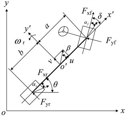
The vehicle state estimation model is established based on a 3-DOF vehicle model.

The dynamic equation of the 3-DOF vehicle model is as follows [16]:

1

{\dot{ω}}_{r} = \frac{a^{2} k_{1} + b^{2} k_{2}}{I_{z}} \frac{ω_{r}}{u} + \frac{a k_{1} - b k_{2}}{I_{z}} β - \frac{a k_{1}}{I_{z}} δ,

2

\dot{β} = \frac{a k_{1} - b k_{2} - m u^{2}}{m} \frac{ω_{r}}{u^{2}} + \frac{k_{1} + k_{2}}{m} \frac{β}{u} - \frac{k_{1} δ}{m u},

3

\dot{u} = a_{x} + v r,

4

a_{y} = \frac{a k_{1} - b k_{2}}{m u} ω_{r} + \frac{k_{1} + k_{2}}{m} β - \frac{k_{1}}{m} δ .

The side slip angle of the center of mass is:

5

β = a r c t a n (\frac{v}{u}) .

Fig. 13-DOF vehicle model

2.2. Tire model

The lateral forces of front and rear wheels can be expressed as [16]:

6

\{\begin{array}{l} F_{y f} = c_{f} α_{f}, \\ F_{y r} = c_{r} α_{r}, \end{array}

where $c_{f}$ and $c_{r}$ are the lateral stiffness of the front and rear tires. $α_{f}$ and $α_{r}$ are the front and rear slip angles:

7

\{\begin{array}{l} c_{f} = \frac{\partial F_{y f}}{\partial α_{f}}| α_{f} = 0, \\ c_{r} = \frac{\partial F_{y r}}{\partial α_{r}}| α_{r} = 0 . \end{array}

3. Adaptive iterative cubature Kalman filter algorithm based on improved maximum correlation entropy

3.1. Maximum correlation entropy criterion

For any two random variables $X$ and $Y$ , the maximum correlation entropy can be defined as [17]:

8

V_{σ} (X, Y) = E [G_{σ} (X - Y)] = \iint_{x, y} G_{σ} (x - y) d F_{X, Y} (x, y),

where $E [\cdot]$ is the expectation operator; $F_{X, Y} (x, y)$ is the joint probability density function; $G_{σ} [\cdot]$ is the kernel function that satisfies the Mercer theorem and has a kernel width of $σ$ . Due to the infinite approximation ability of Gaussian kernel function on nonlinear models, the article adopts the Gaussian kernel function which is expressed as:

9

G_{σ} (x - y) = e^{- \frac{{‖x - y‖}^{2}}{2 σ^{2}}} .

3.2. Improved maximum correlation entropy cubature Kalman filter

Compared to the traditional maximum correlation entropy, the paper combines MCC and WLS and incorporates them into the CKF algorithm to form an improved maximum correlation entropy cubature Kalman filter (IMCC-CKF), which has good convergence, high accuracy, and stability. On the one hand, the MCC criterion is used to handle non-Gaussian noise, and the high-order information of non-Gaussian noise is characterized by introducing Gaussian kernel functions; On the other hand, WLS plays a corrective role in the model by introducing the measurement noise covariance matrix and prior error covariance matrix into the maximum correlation entropy criterion to modify the cost function, further improving the estimation accuracy of vehicle states.

The IMCC-CKF algorithm includes two steps: time update and measurement update. The specific implementation steps are as follows.

Before the algorithm iteration begins, a series of parameters need to be initialized, so the initial state values $x_{0}$ and initial values $P_{0}$ of the error covariance matrix are defined.

Step 1. Time update: The cubature points are generated from state estimation values ${\hat{x}}_{k - 1}$ and error covariance matrix estimation values $P_{k - 1}$ :

10

\{\begin{array}{l} S_{k - 1} = c h o l (P_{k - 1}), \\ x_{k - 1}^{(i)} = S_{k - 1} ζ_{i} + {\hat{x}}_{k - 1}, \end{array}

where $c h o l (\cdot)$ is the Cholesky decomposition; $S_{k - 1}$ is obtained by the Cholesky decomposition of $P_{k - 1}$ ; $x_{k - 1}^{(i)}$ is the $i$ th cubature point at time $k - 1$ , $i = 1,2, \dots, 2 n$ ; $ζ_{i}$ is the cubature point set which is expressed as:

11

ζ_{i} = \{\begin{array}{l} \sqrt{n} [δ]_{i}, i = 1,2, \dots, n, \\ - \sqrt{n} [δ]_{i}, i = n + 1, n + 2, \dots, 2 n, \end{array}

where $[δ]_{i}$ is the $i$ th cubature point which is expressed as $[δ]_{i} = [\begin{array}{l} I_{n} & - I_{n} \end{array}]$ ; $I_{n}$ is the $n \times n$ Identity matrix.

The cubature point $x_{k ∣ k - 1}^{* (i)}$ propagated by the nonlinear state function $f (\cdot)$ is:

12

x_{k ∣ k - 1}^{* (i)} = f (x_{k - 1}^{(i)}) .

The prior state value ${\hat{x}}_{k ∣ k - 1}$ is expressed as:

13

{\hat{x}}_{k ∣ k - 1} = \frac{1}{2 n} \overset{2 n}{\sum_{i = 1}} x_{k ∣ k - 1}^{* (i)} .

The prior error covariance matrix $P_{k ∣ k - 1}$ is expressed as:

14

P_{k ∣ k - 1} = \frac{1}{2 n} \overset{2 n}{\sum_{i = 1}} x_{k ∣ k - 1}^{* (i)} x_{k ∣ k - 1}^{* (i) T} - {\hat{x}}_{k ∣ k - 1} {\hat{x}}_{k ∣ k - 1}^{T} + Q_{k - 1} .

Step 2. Measurement update: Cubature point sampling again through ${\hat{x}}_{k ∣ k - 1}$ and $P_{k ∣ k - 1}$ :

15

\{\begin{array}{l} S_{k ∣ k - 1} = c h o l (P_{k ∣ k - 1}), \\ x_{k ∣ k - 1}^{(i)} = S_{k ∣ k - 1} ζ_{i} + {\hat{x}}_{k ∣ k - 1} . \end{array}

The expressions of the transform value and predicted measurement value of the cubature point are as follows:

16

z_{k ∣ k - 1}^{(i)} = h (x_{k ∣ k - 1}^{(i)}),

17

{\hat{z}}_{k ∣ k - 1} = \frac{1}{2 n} \sum_{i = 1}^{2 n} z_{k ∣ k - 1}^{(i)},

where $z_{k ∣ k - 1}^{(i)}$ is the quadratic propagation of the nonlinear measurement function $h (\cdot)$ on the cubature point.

The covariance matrix of the predicted measurement error is equal to:

18

P_{z z, k ∣ k - 1} = \frac{1}{2 n} \overset{2 n}{\sum_{i = 1}}  z_{k ∣ k - 1}^{(i)} z_{k ∣ k - 1}^{(i) T} - {\hat{z}}_{k ∣ k - 1} {\hat{z}}_{k |k - 1}^{T} + R_{k - 1} .

The covariance matrix $P_{x z, k ∣ k - 1}$ of the predicted measurement error is equal to:

19

P_{x z, k ∣ k - 1} = \frac{1}{2 n} \sum_{i = 1}^{2 n} x_{k ∣ k - 1}^{(i)} z_{k ∣ k - 1}^{(i) T} - {\hat{x}}_{k ∣ k - 1} {\hat{z}}_{k ∣ k - 1}^{T} .

The pseudo measurement matrix $H_{k}$ is obtained as follows:

20

H_{k} = P_{x z, k ∣ k - 1}^{T} P_{k ∣ k - 1}^{- 1} .

Then the measurement function can be approximated as:

21

z_{k} \approx h ({\hat{x}}_{k ∣ k - 1}) + \frac{\partial h}{\partial x_{k}} ∣_{x_{k} = {\hat{x}}_{k ∣ k - 1}} (x_{k} - {\hat{x}}_{k ∣ k - 1}) + v_{k} \approx {\hat{z}}_{k ∣ k - 1} + H_{k} (x_{k} - {\hat{x}}_{k ∣ k - 1}) + v_{k} .

Combining WLS with Gaussian kernel involves adding relevant weight matrices $R_{k}^{- 1}$ and $P_{k ∣ k - 1}$ to the Gaussian kernel function. The cost function of the Gaussian kernel function based on the weight matrix is:

22

J_{M C C} (x_{k}) = G_{σ} ({‖x_{k} - {\hat{x}}_{k ∣ k - 1}‖}_{(P_{k ∣ k - 1}^{- 1})}^{2}) + G_{σ} ({‖z_{k} - {\hat{z}}_{k ∣ k - 1} - H_{k} (x_{k} - {\hat{x}}_{k ∣ k - 1})‖}_{R_{k}^{- 1}}^{2}),

where ${‖\cdot‖}_{A}^{2} = (\cdot)^{T} A (\cdot)$ is the weighted squared Mahalanobis distance of vector $A$ . The Gaussian kernels with squared Mahalanobis distance are redefined as:

23

G_{σ} ({‖\cdot‖}_{A}^{2}) = e^{- \frac{{‖\cdot‖}_{A}^{2}}{2 σ^{2}}} .

The optimal estimation of ${\hat{x}}_{k}$ obtained by maximizing the objective function is:

24

{\hat{x}}_{k} = \underset{x_{k}}{a r g m a x} J_{M C C} (x_{k}) .

In response to the difficulty in obtaining analytical solutions for the optimization problem mentioned above, the iterative Gaussian-Newton method based on gradient descent is used to solve the above equation, and the state vector equation at time $k$ is obtained as follows:

25

{\hat{x}}_{k |k}^{i t} = {\hat{x}}_{k |k - 1} + {\bar{K}}_{k}^{i t} (z_{k} - H_{k} ({\hat{x}}_{k |k - 1}^{i t}) - {\bar{H}}_{k}^{i t} ({\hat{x}}_{k |k - 1} - {\hat{x}}_{k |k}^{i t - 1})),

where:

26

{\bar{H}}_{k}^{i t} = (P_{x y, k}^{i t})^{T} P_{k |k - 1}^{- 1},

27

{\hat{R}}_{k}^{i t} = (P_{y y, k}^{i t})^{T} - {\bar{H}}_{k}^{i t} P_{k |k - 1}^{- 1} ({\bar{H}}_{k}^{i t})^{T},

28

{\bar{K}}_{k}^{i t} = [L_{r}^{i t} ({\bar{H}}_{k}^{i t})^{T} {\bar{R}}_{k}^{i t} {\bar{H}}_{k}^{i t} + L_{q}^{i t} P_{k |k - 1}^{- 1}]^{- 1} \cdot L_{r}^{i t} ({\bar{H}}_{k}^{i t})^{T} ({\bar{R}}_{k}^{i t})^{- 1},

29

L_{r}^{i t} = G_{σ} ({‖z_{k} - H_{k} x_{k}‖}_{R_{k}^{- 1}}) |_{x_{k} = {\hat{x}}_{k}^{i t - 1}},

30

L_{q}^{i t} = G_{σ} ({‖x_{k} - {\hat{x}}_{k |k - 1}‖}_{P_{k |K - 1}^{- 1}}) |_{x_{k} = {\hat{x}}_{k}^{i t - 1}} .

The covariance matrix $P_{k}^{i t}$ of state estimation error is calculated as:

31

P_{k}^{i t} = (I - {\bar{K}}_{k}^{i t} {\bar{H}}_{k}^{i t}) P_{k |k - 1} (I - {\bar{K}}_{k}^{i t} {\bar{H}}_{k}^{i t})^{T} + {\bar{K}}_{k}^{i t} {\bar{R}}_{k}^{i t} ({\bar{K}}_{k}^{i t})^{T} .

The state vector $x$ and covariance matrix $P$ after $j$ iterations are calculated are as follows:

32

{\hat{x}}_{k} = {\hat{x}}_{k}^{j},

33

P_{k} = P_{k}^{j} .

Gaussian kernel plays an important role in any entropy filtering algorithm. In Eqs. (29)-(30), the smaller the values of $σ$ are, the smaller the gain ${\bar{K}}_{k}^{i t}$ will be. Under Gaussian noise, the filtering performance may decrease or even diverge. In real-world applications, the Gradient descent optimization method which firstly initializes $σ$ as the global median distance and then use backpropagation or Bayesian optimization to adjust $σ$ is used to determine $σ$ . At the same time, the weights $L_{r}^{i t}$ and $L_{q}^{i t}$ are used to adjust the gain ${\bar{K}}_{k}^{i t}$ , and there is no need to invert the diagonal matrix containing error indices, effectively avoiding the numerical problem of algorithm failure caused by encountering large observation errors.

Due to the varying optimal kernel sizes in different noise environments, it is necessary to improve the adaptive method for kernel size. Appropriate kernel size is crucial for improving robustness and performance.

3.3. Improved algorithm of maximum correlation entropy for adaptive iterative cubature Kalman filter

The application of a covariance matrix of fixed process and measurement noise can lead to estimation errors and make it difficult to meet practical needs. Therefore, based on the IMCC-CKF algorithm, adaptive and iterative methods are further adopted to improve the accuracy of the algorithm. The role of WLS is to minimize the estimated variance by adjusting the weighting matrix. The combination of these two will result in constructing a new objective function. Meanwhile, the AICKF can adjust the filter gain and covariance matrix in real-time based on the current measurement situation.

In order to better adapt to external dynamic interference, the article further improves the accuracy and stability of the algorithm by adaptively adjusting the covariance matrices of process and measurement noise.

In this algorithm, the information from the observed residual sequence is applied to adaptively update the noise covariance matrix, instead of using a fixed noise covariance matrix for recursive estimation to improve the estimation accuracy of the algorithm. The specific calculation method is as follows:

The residual of the relevant output observation vector is calculated as:

34

v_{k} = z_{k} - {\hat{z}}_{k |k - 1} .

The residual covariance matrix of the relevant output observation vector is calculated as:

35

E_{k} = \frac{1}{M} \overset{k}{\sum_{j = k - M + 1}} e_{j} (e_{j})^{T} .

The covariance matrix of the process noise at time $k +$ 1 is updated as follows:

36

Q_{k + 1} = {\bar{K}}_{k}^{j} E_{k} ({\bar{K}}_{k}^{j})^{T} .

The covariance matrix of the observation noise at time $k +$ 1 is updated as follows:

37

R_{k + 1} = E_{k} + \sum_{i = 0}^{2 n} w_{c}^{i} [z_{k |k - 1}^{(i)} - {\hat{z}}_{k ∣ k - 1}] [z_{k |k - 1}^{(i)} - {\hat{z}}_{k ∣ k - 1}]^{T} .

By combining the improved maximum correlation entropy cubature Kalman filter with iterative optimization and adaptive adjustment, the accuracy can be improved while maintaining the algorithm efficiency.

4. Numerical simulation and experimental verification

This article uses the IMCC-AICKF method to filter and estimate the yaw rate and side slip angle as well as the longitudinal velocity. A Carsim and Matlab/Simulink joint simulation platform is established for simulation, and the results are compared and analyzed with traditional cubature Kalman filter simulation.

4.1. Numerical simulation

4.1.1. Double-lane change condition

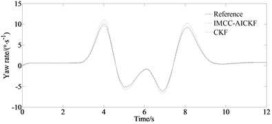
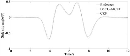
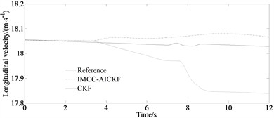
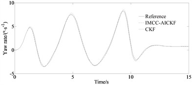
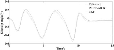
The simulation results of the yaw rate and side slip angle as well as longitudinal velocity of the vehicle under the double-lane change condition are shown in Fig. 2.

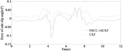
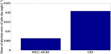
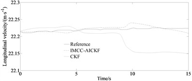
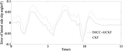
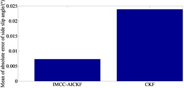
From Figs. 2(a)-(b), it can be seen that compared to the traditional CKF algorithm, the filter estimation values of the IMCC-AICKF algorithm can better approach the reference values. And the deviation at the peaks and valleys of the curve is relatively small, and it has a significant noise suppression effect. From Fig. 2(c), it can be seen that under the double-lane change condition, the longitudinal velocity estimation value of the IMCC-AICKF algorithm finally converge to the reference value and is significantly closer to the reference value than the traditional CKF algorithm that leads to a faster convergence speed and higher computational efficiency. In the case of unknown noise conditions, the IMCC-AICKF algorithm has a stronger noise suppression effect and better stability and robustness. From Fig. 2(d)-(e), it can be seen that the error of side slip angle of the IMCC-AICKF algorithm is smaller than that of the CKF algorithm indicating the higher estimation accuracy of the proposed algorithm. This is because the proposed method uses the MCC algorithm to process measurement noise. And the values of adaptive factors are determined from different measurement environments, and the covariance matrix of the observed noise is adjusted online through the adaptive factors, thereby completing the estimation of the state and real-time update of the covariance. The IMCC-AICKF algorithm can effectively suppress non-Gaussian noise and ultimately exhibit relatively high convergence accuracy, demonstrating the advantages of the IMCC-AICKF algorithm in dealing with non-Gaussian noise problems.

Fig. 2Simulation results under double-lane change condition: a) yaw rate; b) side slip angle; c) longitudinal velocity; d) error of side slip angle; e) mean of absolute error of side slip angle

Simulation results under double-lane change condition: a) yaw rate; b) side slip angle; c) longitudinal velocity; d) error of side slip angle; e) mean of absolute error of side slip angle

a)

b)

c)

d)

e)

4.1.2. Serpentine condition

The simulation results of the yaw rate and side slip angle as well as longitudinal velocity of the vehicle under the serpentine condition are shown in Fig. 3.

From Figs. 3(a)-(b), it can be seen that at the peaks and valleys of the curve, compared to the traditional CKF algorithm, the IMCC-AICKF algorithm can better approach the reference value, with relatively small deviations and strong suppression of noise fluctuations. From Fig. 3(c), it can be seen that under the serpentine condition, the longitudinal velocity estimation value of the IMCC-AICKF algorithm finally converge to the reference value and is significantly closer to the reference value than the traditional CKF algorithm that indicates at a faster convergence speed and higher computational efficiency. In the case of unknown noise conditions, the IMCC-AICKF algorithm has a stronger noise suppression effect and better stability and robustness. From Fig. 3(d)-(e), it can be seen that the error of side slip angle of the IMCC-AICKF algorithm is smaller than that of the CKF algorithm demonstrating the higher estimation accuracy of the proposed algorithm. On the one hand, the MCC criterion is used to handle non-Gaussian noise, and the high-order information of non-Gaussian noise is characterized by introducing Gaussian kernel functions. On the other hand, the WLS plays a corrective role in the model by introducing the measurement noise covariance matrix and prior error covariance matrix into the maximum correlation entropy criterion to modify the cost function, further improving the accuracy of vehicle state estimation. Meanwhile, the IMCC-AICKF algorithm combines adaptive factors with an improved maximum correlation entropy criterion, enhancing the adaptability of the algorithm.

Fig. 3Simulation results under serpentine condition: a) yaw rate; b) side slip angle; c) longitudinal velocity; d) error of side slip angle; e) mean of absolute error of side slip angle

Simulation results under serpentine condition: a) yaw rate; b) side slip angle; c) longitudinal velocity; d) error of side slip angle; e) mean of absolute error of side slip angle

a)

b)

c)

d)

e)

4.2. Sensitivity analysis

A sensitivity analysis demonstrating the algorithm performance under varying noise levels and different road conditions was made.

The root mean square error (RMSE) under varying noise levels and different road conditions are shown in Table 1 and Table 2. The expressions of the indicators are as follows:

38

R M S E (x) = \sqrt{\frac{\sum_{k = 1}^{N} {(x_{k | k} - x_{a c t u a l} (k))}^{2}}{N}},

where $x_{k | k}$ and $x_{a c t u a l} (k)$ are the estimated and the real value at time $k$ respectively.

Table 1 is the RMSE of the estimated parameters (Side slip angle) for two algorithms under different road conditions.

From Table 1, it can be seen that the RMSE value of the estimation parameters of IMCC-AICKF is smaller than that of the CKF algorithm. This indicates that the IMCC-AICKF algorithm can effectively suppress non-Gaussian noise interference and has high estimation accuracy. This is mainly because the CKF algorithm is based on the MSE criterion, which is more sensitive to larger outliers in non-Gaussian noise environments. The IMCC-AICKF algorithm is based on the MC criterion, which can capture high-order statistics in non-Gaussian distributions. Appropriate kernel width parameters, if selected, can effectively suppress outliers in non-Gaussian noise and achieve high estimation accuracy. The RMSE of both algorithms under the slalom road condition is greater than that under the double-lane change road condition, due to the significant curvature variation of the slalom road. At the same time, the IMCC-AICKF algorithm can quickly converge to the actual value under different operating conditions, and its accuracy is still higher than CKF, which verifies that the IMCC-AICKF algorithm can estimate the vehicle state with higher accuracy under different operating conditions, reflecting the effectiveness and robustness of the algorithm.

Table 2 is the RMSE of the estimation parameters (Side slip angle) of two algorithms under different initial values of the covariance matrix of measurement noise.

Table 1Analysis of estimation errors of states under different road conditions

Side slip angle	Double-lane change road		Slalom road
Side slip angle	IMCC-AICKF	CKF	IMCC-AICKF	CKF
RMSE	0.00132	0.00301	0.00156	0.00352

Table 2Analysis of estimation errors of states under different initial conditions of measurement noise covariance matrix

$u$		Initial value of $R$
$u$		$e y e (3) \times 0.01$	$e y e (3) \times 2$
RMSE	IMCC-AICKF	0.001	0.003
RMSE	CKF	0.002	0.081

Table 2 shows that when the initial value of the measurement noise covariance matrix is $R_{0}$ = eye(3)×0.01, the estimation accuracy of IMCC-AICKF for the side slip angle is improved by 50 % compared to CKF. When the initial value of the measurement noise covariance matrix is set to $R_{0}$ = eye(3)×2, the estimation accuracy of the side slip angle after using the IMCC-AICKF is improved by 96 % compared to CKF. This indicates that CKF is very sensitive to the initial value of the covariance matrix of measurement noise, which is also the reason why it is difficult to ensure the estimation accuracy of CKF in practical applications. The IMCC-AICKF algorithm proposed in this paper not only improves the estimation accuracy but also has strong robustness.

In summary, the IMCC-AICKF proposed in this article has significant advantages in estimation accuracy.

4.3. Experimental verification

A virtual test using the CarSim software is conducted to verify the feasibility of the simulated results.

CarSim is a simulation software specifically developed for vehicle dynamics. This software enjoys a high reputation both internationally and domestically, and is adopted by numerous automobile manufacturers and component suppliers. The main user interface of CarSim software consists of two modules: scalable graphical user interface (SGUI) and graphical data management system. Its model runs 3-6 times faster in a computer simulation than in the real-time measurements. In the database, parameters such as road environment information, driver model, vehicle model, and aerodynamic response can be set. The CarSim simulation platform has the advantages of accuracy, convenience, good visualization, high cost-effectiveness and real-time monitoring, and has good practicality for the study.

At the same time, this paper conducted real an experimental verification research for a vehicle. The real experimental vehicle is shown in Fig. 4. The measurement devices are shown in Fig. 5.

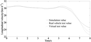
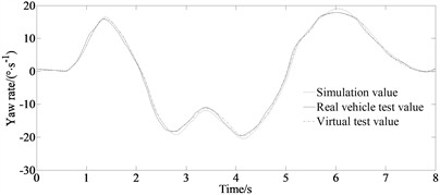
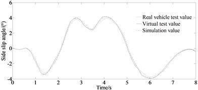
The experimental results of the longitudinal velocity and yaw rate as well as side slip angle of the vehicle under the double lane changing condition are shown in Fig. 6.

Fig. 4Real test vehicle

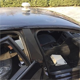
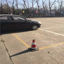
Fig. 5Measurement devices

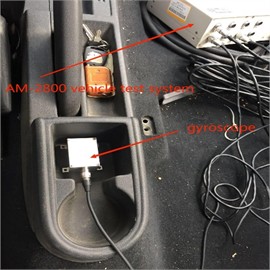
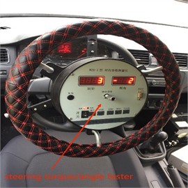
Fig. 6Experimental results: a) longitudinal velocity; b) yaw rate; c) side slip angle

a)

b)

c)

It can be seen that the results of the virtual test and the simulation value do not coincide. This is because the model in the virtual test ignored the nonlinearity of the steering and suspension systems. And this explains the inconsistency between the virtual test value and the real vehicle test value. And the model error increased by about 4.99 %, 3.92 % and 3.59 % for the longitudinal velocity, yaw rate and side slip angle compared with the corresponding real vehicle test values. However, compared to the traditional maximum correlation entropy studies, this paper combines the MCC and WLS, and incorporates them into the CKF algorithm to form an improved maximum correlation entropy volume Kalman filter to improve the robustness of the filtering algorithm in measuring abnormal situations. And the Gaussian kernel function is used as the adjustment factor for correlation entropy. The adaptive factors are selected according to different measurement environments and the covariance matrix of observation noise is adjusted to achieve good convergence, high accuracy, and stability. So, the trends of the curves of both the test values and the simulation values are sufficient to illustrate the correctness of the proposed method.

5. Conclusions

Based on the advantages of AICKF algorithm and maximum correlation entropy as well as weighted least squares theory, this article applies an improved maximum correlation entropy adaptive iterative cubature Kalman Filter algorithm to estimate the vehicle state under non-Gaussian noise. In order to verify the effectiveness and accuracy of the IMCC-AICKF algorithm, simulation experiments are designed under two different operating conditions: double-lane change condition and serpentine condition. The simulation results show that the IMCC-AICKF algorithm had better filtering estimation performance for yaw rate, side slip angle and longitudinal velocity under both conditions. In the case of unknown noise conditions, the IMCC-AICKF algorithm had stronger noise suppression effect, better stability, and robustness. The virtual results showed that the proposed algorithm could better estimate states of vehicles and had good robustness, improving the accuracy of the filtering algorithm and enhancing its adaptability. The algorithm proposed in this article can improve the accuracy of vehicle state estimation in non-Gaussian noise environments and has good robustness, providing effective technical support for the practical application of intelligent vehicle state estimation.

The weight matrix of the weighted least squares part needs to be adaptively adjusted according to the noise characteristics, and improper selection can lead to performance degradation. Therefore, in the future, the adaptive adjustment method of the weight matrix in the weighted least squares part need to be researched.

References

Y. Liu, D. Cui, and W. Peng, “Optimum control for path tracking problem of vehicle handling inverse dynamics,” Sensors, Vol. 23, No. 15, p. 6673, Jul. 2023, https://doi.org/10.3390/s23156673

Publisher
Y. Liu, D. Cui, and W. Peng, “Optimal lane changing problem of vehicle handling inverse dynamics based on mesh refinement method,” IEEE Access, Vol. 11, pp. 115617–115626, Jan. 2023, https://doi.org/10.1109/access.2023.3324422

Publisher
Y. Liu and D. Cui, “Vehicle dynamics prediction via adaptive robust unscented particle filter,” Advances in Mechanical Engineering, Vol. 15, No. 5, p. 168781322311707, May 2023, https://doi.org/10.1177/16878132231170766

Publisher
J. Geng, L. Xia, and D. Wu, “Attitude and heading estimation for indoor positioning based on the adaptive cubature Kalman filter,” Micromachines, Vol. 12, No. 1, p. 79, Jan. 2021, https://doi.org/10.3390/mi12010079

Publisher
L. Li, D. Yu, Y. Xia, and H. Yang, “Event‐triggered UKF for nonlinear dynamic systems with packet dropout,” International Journal of Robust and Nonlinear Control, Vol. 27, No. 18, pp. 4208–4226, Mar. 2017, https://doi.org/10.1002/rnc.3790

Publisher
S. Huang, C. Chao, J. Huang, and Y. Lv, “Parameter estimation of unmanned vehicle based on ESO and EKF algorithm,” in Lecture Notes in Electrical Engineering, pp. 469–476, Jun. 2024, https://doi.org/10.1007/978-981-97-3332-3_42

Publisher
J. Bao, Z. Lin, H. Jing, H. Feng, X. Zhang, and Z. Luo, “Research on longitudinal control of electric vehicle platoons based on robust UKF-MPC,” Sustainability, Vol. 16, No. 19, p. 8648, Oct. 2024, https://doi.org/10.3390/su16198648

Publisher
Y. Liu, D. Cui, and W. Peng, “Vehicle state and parameter estimation based on adaptive robust unscented particle filter,” Journal of Vibroengineering, Vol. 25, No. 2, pp. 392–408, Mar. 2023, https://doi.org/10.21595/jve.2022.22788

Publisher
D. X. Xing, M. X. Wei, and W. Z. Zhao, “Vehicle state estimation based on adaptive cubature particle filtering,” Journal of Nanjing University of Aeronautics and Astronautics, Vol. 52, No. 3, pp. 445–453, Mar. 2020, https://doi.org/10.16356/j.1005-2615.2020.03.013

Publisher
T. Chen et al., “Design and verification for vehicle longitudinal force and sideslip angle hierarchical estimation method,” Journal of Xi’an Jiaotong University, Vol. 53, No. 11, pp. 131–140, 2019, https://doi.org/10.7652/xjtuxb201911019

Publisher
T. Chen, L. Chen, X. Xu, Y. Cai, H. Jiang, and X. Sun, “Sideslip angle fusion estimation method of an autonomous electric vehicle based on robust cubature Kalman filter with redundant measurement information,” World Electric Vehicle Journal, Vol. 10, No. 2, p. 34, May 2019, https://doi.org/10.3390/wevj10020034

Publisher
X. Chen and X. Cheng, “RBCKF-based vehicle state estimation by adaptive weighted fusion strategy considering composite-state tire model,” World Electric Vehicle Journal, Vol. 15, No. 11, p. 517, Nov. 2024, https://doi.org/10.3390/wevj15110517

Publisher
Y. Wei, X. Yang, X. Bai, and Z. Xu, “Adaptive hybrid Kalman filter for attitude motion parameters estimation of space non-cooperative tumbling target,” Aerospace Science and Technology, Vol. 144, p. 108832, Jan. 2024, https://doi.org/10.1016/j.ast.2023.108832

Publisher
P. Dahal, S. Mentasti, L. Paparusso, S. Arrigoni, and F. Braghin, “RobustStateNet: robust ego vehicle state estimation for autonomous driving,” Robotics and Autonomous Systems, Vol. 172, p. 104585, Feb. 2024, https://doi.org/10.1016/j.robot.2023.104585

Publisher
F. Lin et al., “Road friction coefficient estimation based on improved Keras model,” Journal of Mechanical Engineering, Vol. 57, No. 12, pp. 74–86, Jan. 2021, https://doi.org/10.3901/jme.2021.12.074

Publisher
Y. Liu, D. Cui, and W. Peng, “Vehicle state and parameter estimation based on improved extend Kalman filter,” Journal of Measurements in Engineering, Vol. 11, No. 4, pp. 496–508, Dec. 2023, https://doi.org/10.21595/jme.2023.23475

Publisher
C. L. Wu et al., “Estimation of lithium-ion battery state of charge using an innovation maximum correlation-entropy criterion adaptive iterative cubature Kalman filter algorithm,” Journal of XI’AN Jiaotong University, Vol. 58, No. 11, pp. 52–64, 2024, https://doi.org/10.7652/xjtuxb202411005

Publisher

About this article

Received

14 January 2025

Accepted

01 May 2025

Published

01 June 2025

DOI

https://doi.org/10.21595/jme.2025.24792

Keywords

automotive engineering

cubature Kalman filter

iterative maximum correntropy criterion

maximum correlation entropy

vehicle state estimation

Acknowledgements

This research was supported by the Open Research Program of Huzhou Key Laboratory of Urban Multidimensional Perception and Intelligent Computing under Grant No. UMPIC202404.

Data Availability

The datasets generated during and/or analyzed during the current study are available from the corresponding author on reasonable request.

Author Contributions

Yingjie Liu: mathematical model and the simulation techniques. Dawei Cui: spelling and grammar checking as well as software. Chenglian Xie: virtual validation.

Conflict of interest

The authors declare that they have no conflict of interest.

This is an open access article distributed under the Creative Commons Attribution License, which permits unrestricted use, distribution, and reproduction in any medium, provided the original work is properly cited.

Research article

2025 01 02

Estimation of vehicle state based on maximum correntropy square-root cubature Kalman Filter

Yingjie Liu, Dawei Cui

Research article

2023 11 18

Vehicle state and parameter estimation based on adaptive anti-outlier unscented Kalman filter and GA-BPNN method

Yingjie Liu, Dawei Cui, Wen Peng

Research article

2023 10 30

Vehicle state and parameter estimation based on improved extend Kalman filter

Yingjie Liu, Dawei Cui, Wen Peng

Research article

2023 09 21

Defect identification in electro-mechanical assembly using finite element method and modal assurance criterion

Rishabh Singh, Amogh R. Nalawade, Matthew Pieczko

Y. Liu, D. Cui, and C. Xie, “Measurement and estimation of vehicle state based on improved maximum correntropy square-root cubature Kalman filter,” Journal of Measurements in Engineering, Vol. 13, No. 3, –13, Jun. 2025, https://doi.org/10.21595/jme.2025.24792

Copy Extrica

Copied to clipboard!

TY  - JOUR
DO  - 10.21595/jme.2025.24792
UR  - https://doi.org/10.21595/jme.2025.24792
TI  - Measurement and estimation of vehicle state based on improved maximum correntropy square-root cubature Kalman filter
T2  - Journal of Measurements in Engineering
AU  - Liu, Yingjie
AU  - Cui, Dawei
AU  - Xie, Chenglian
PY  - 2025
DA  - 2025/06/01
PB  - Extrica
VL  - 13
IS  - 3
SN  - 2335-2124
SN  - 2424-4635
ER  - 

Copy Ris

Copied to clipboard!

 @article{Liu_2025, title={Measurement and estimation of vehicle state based on improved maximum correntropy square-root cubature Kalman filter}, ISSN={2424-4635}, url={https://doi.org/10.21595/jme.2025.24792}, DOI={10.21595/jme.2025.24792}, journal={Journal of Measurements in Engineering}, publisher={JVE International Ltd.}, author={Liu, Yingjie and Cui, Dawei and Xie, Chenglian}, year={2025}, month=jun }

Copy Bibtex

Copied to clipboard!

[1]Y. Liu, D. Cui, and C. Xie, “Measurement and estimation of vehicle state based on improved maximum correntropy square-root cubature Kalman filter,” Journal of Measurements in Engineering, Jun. 2025, doi: 10.21595/jme.2025.24792.

Copy IEEE

Copied to clipboard!

Liu, Yingjie, Dawei Cui, and Chenglian Xie. “Measurement and Estimation of Vehicle State Based on Improved Maximum Correntropy Square-Root Cubature Kalman Filter.” Journal of Measurements in Engineering, June 1, 2025. https://doi.org/10.21595/jme.2025.24792.

Copy Chicago

Copied to clipboard!

Measurement and estimation of vehicle state based on improved maximum correntropy square-root cubature Kalman filter

Abstract

Highlights

1. Introduction

2. Mathematical model of vehicle state estimation problem

2.1. 3-DOF vehicle model

2.2. Tire model

3. Adaptive iterative cubature Kalman filter algorithm based on improved maximum correlation entropy

3.1. Maximum correlation entropy criterion

3.2. Improved maximum correlation entropy cubature Kalman filter

3.3. Improved algorithm of maximum correlation entropy for adaptive iterative cubature Kalman filter

4. Numerical simulation and experimental verification

4.1. Numerical simulation

4.1.1. Double-lane change condition

4.1.2. Serpentine condition

4.2. Sensitivity analysis

4.3. Experimental verification

5. Conclusions

References

About this article

Related Articles