Application of statistical modelling method for determination of optimal solutions of road transport problems

Tulenov, Aidarali; Baubekov, Yermek; Shoibekov, Baurzhan; Bakyt, Gabit; Bekbolatov, Gabit; Ablyalimov, Oleg

doi:10.21595/vp.2025.25012

Vibroengineering Procedia

Browse Procedia

Published: 15 May 2025

Check for updates

Application of statistical modelling method for determination of optimal solutions of road transport problems

Aidarali Tulenov¹

Yermek Baubekov²

Baurzhan Shoibekov³

Gabit Bakyt⁴

Gabit Bekbolatov⁵

Oleg Ablyalimov⁶

^{1, 3, 5}M. Auezov South Kazakhstan University, Shymkent, Kazakhstan

^{2, 4}Mukhametzhan Tynyshbayev ALT University, Almaty, Kazakhstan

⁶Tashkent State Transport University, Tashkent, Uzbekistan

Corresponding Author:

Gabit Bakyt

Cite the article Download PDF

Downloads 175

Abstract

The article is devoted to the use of statistical modelling to solve problems related to the functioning of road transport and mass service systems, such as car service stations. The method consists in reproducing the process under study using a probabilistic mathematical model and subsequent statistical processing of data to obtain numerical characteristics of the process. The purpose of the study is to apply the method of statistical modelling to determine optimal solutions to problems such as calculating the probability of system states, the average number of occupied channels, queuing time and other characteristics of the service station. A station with two service channels and two waiting places is considered as an object of research. The methods of probability theory, including the law of large numbers and Bernoulli's theorem, have been used to solve the set tasks. The modelling results show that in the process of station operation the probability of failure and other characteristics, such as average waiting time, can be accurately calculated using a statistical approach. The main research method is random variable modelling using uniformly distributed random numbers and their logarithmic transformations to simulate application arrival times and service times. The conclusions of the study confirm the high efficiency of the method of statistical modelling for the analysis and optimization of transport systems and mass service systems, as well as its possible application for other tasks, such as determining the capacity of transport interchanges, reliability of technical systems and other logistic processes.

Application of statistical modelling method for determination of optimal solutions of road transport problems

Highlights

It has been established that the statistical modeling method is an effective approach for solving problems arising in the transport industry.
The effectiveness of the statistical modeling method has been proven by using random numbers.
A graph has been constructed to calculate the state time of the queuing system with different numbers of channels.
It is proved that the statistical modeling method can be used to determine the capacity of transport and logistics centers and specialized posts, etc.

1. Introduction

Modern transportation systems require process optimization to increase their efficiency and reliability. One of the methods to achieve this goal is statistical modeling based on probabilistic and mathematical models. This study examines the application of the statistical modeling method to solve problems related to the functioning of motor transport, namely, to analyze and optimize the operation of car service stations. The main task is to determine the numerical characteristics of the functioning of such systems, including the probability of system states, waiting time, and the average number of busy service channels. The use of statistical modeling allows not only to evaluate the efficiency of existing systems, but also to propose solutions to improve their performance [1, 2].

The purpose of the article is to substantiate the effectiveness of the statistical modeling method for solving applied problems in the field of motor transport, using the example of using random numbers to optimize routes, load planning, forecasting the technical condition of vehicles and increasing the economic efficiency of transportation.

The scientific novelty of this work lies in the development and adaptation of a statistical model that takes into account a complex set of factors affecting the efficiency of motor transport, including variable loads, road and climatic conditions, operating modes and the technical condition of the fleet. Unlike existing approaches, the proposed method allows for the integration of stochastic parameters and the use of real statistical data to form optimal management decisions. The novelty also lies in the application of statistical modeling to assess the sustainability of transport solutions under changing external conditions and incomplete initial information, which expands the possibilities of forecasting and optimization in transport logistics [3, 4].

The developed methodology makes it possible to more accurately determine optimal routes, traffic schedules, loading of rolling stock and vehicle maintenance strategies. This provides a significant increase in the efficiency of logistics operations, reducing operating costs and increasing the stability of transport processes in conditions of uncertainty.

2. Materials and methods

To solve the tasks set in the article, the statistical modeling method is used, which includes the construction of probabilistic mathematical models of the processes under study and repeated modeling to obtain statistical data. The basis of the method is the law of large numbers, which guarantees the convergence of the average values of the results of a set of independent tests to the mathematical expectation of a random variable. As an example, the car maintenance process at a service station was considered, where the models for the time of receipt of applications and the time of their maintenance are distributed according to an exponential law. Random numbers evenly distributed over the interval 0.1 were used for modeling, which made it possible to generate data for further calculations. Modeling was carried out for several process implementations, followed by statistical data processing to obtain the average characteristics of the system [5].

The statistical modeling method consists in reproducing the physical process under study using a probabilistic mathematical model and calculating the characteristics of this process. This method is based on repeated tests of the constructed model with subsequent statistical processing of the data obtained in order to determine the numerical characteristics of the process under consideration in the form of statistical estimates of its parameters. The basis of the statistical modeling method is the law of higher numbers.

In probability theory, the law of large numbers refers to a number of theorems in which, for certain conditions, convergence in probability of the average values of the results of a large number of observations to certain constant values is proved. For example, one of Chebyshev’s theorems is formulated as follows: With an unlimited increase in the number of independent trials, $n$ , the arithmetic mean, free from systematic errors and equivalent results of observations $x_{i}$ of a quantity $X$ with finite variance $D [x]$ , converges in probability to the mathematical expectation $M [x]$ of a random variable [6, 7]:

1

\lim P \{|\frac{\sum_{i = 1}^{n} x_{i}}{n} - M [x]| < ε\} = 1,

where $ε$ – an arbitrarily small positive value.

Bernoulli’s theorem is formulated as follows: With an unlimited increase in the number of independent trials under the same conditions, the frequency $P^{*} (A)$ of the occurrence of a random event $A$ converges in probability to its probability $P$ i.e.:

2

\lim P \{|\frac{m_{i}^{*}}{n} - P| < ε\} = 1 .

Therefore, in order to obtain the probability of an event, for example, the probabilities of the queuing system state $P (0)$ , $P (1)$ ,…, $P (k)$ , the frequencies $P_{i}^{*} = m_{i}^{*} / n$ are calculated for one implementation. Next, similar calculations are performed for a number equal to, for example, $n =$ 1000. The results are averaged, and thus, with some approximation, the desired probabilities of the system states are obtained. Based on the calculated probabilities $P_{0}^{*}$ , $P_{1}^{*}$ , $P_{2}^{*}$ ,…, $P_{k}^{*}$ ,…, $P_{n}^{*}$ calculate the mathematical expectation of the number of occupied channels $M^{*} [S]$ , the waiting time for the queue $M^{*} [S]$ , the average time spent in the queue $t_{a v e r . t i m e}^{*}$ and other characteristics.

3. Results

Multiple statistical observations [8, 9] have established that the time intervals between two service requests, for example, the time intervals between two cars arriving at a service station (as well as the service time of these requests), are distributed according to an exponential law:

f (t) = λ ∙ e^{- λ t} .

And that means:

y = F (t) = \int_{0}^{t} λ ∙ e^{- λ t} = 1 - e^{- λ t},

or:

3

y = 1 - e^{- λ t}, e^{- λ t} = 1 - y,

where $λ$ – the density or intensity of applications, i.e. the average number of applications per unit of time.

Logarithming the resulting expression, we get:

4

- λ ∙ t ∙ \ln e = \ln (1 - y), t_{i} = - \frac{2,3}{λ} ∙ l g (1 - y_{i}),

where $y_{i}$ – random numbers uniformly distributed in the range [0.1] and stochastically independent.

Thus, the resulting expression is an algorithm for modeling random variables distributed according to an exponential law.

The values of $y_{i}$ are usually obtained from a table of evenly distributed random numbers. To illustrate, Table 1 shows an excerpt from this table.

Table 1A fragment from the table of uniformly distributed random numbers

27	76	74	35	84	85	30	18	89	77	29	49	06	97	14
03	54	51	43	38	54	06	61	52	43	47	72	46	67	33
80	21	73	62	92	98	52	52	43	35	24	43	22	48	96
10	87	56	20	04	90	30	16	11	05	57	41	10	63	68
54	12	75	73	26	26	62	91	90	87	24	47	28	87	78

All the values of the numbers shown in Table 1 are less than one, so when using the table, you must put a zero in front. For example, the first number is 0.27, etc.

The operation of a car service station, which has two channels ( $n =$ 2) and two places to wait in line ( $m =$ 2), is being investigated. The station receives the simplest Poisson flow of applications with a density of $λ =$ 1.5 cars per hour, and the service time of the machines is distributed according to the exponential law and averages $M_{t_{s e r v .}} =$ 2.5 hours per car. Using the statistical modeling method, it is required to determine the numerical characteristics of the station’s operation in one 10-hour working day. When modeling the time of receipt of applications, we will use row 1 of the Table 1, and when modeling the service time, use row 2 of the same table, starting, for example, on the third day [10].

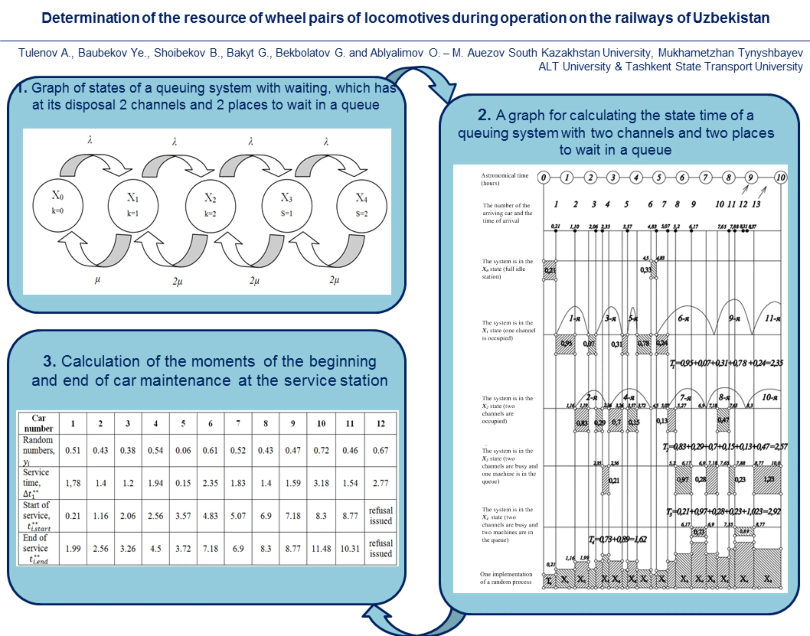
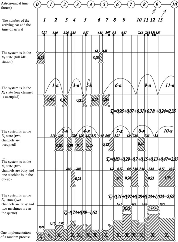
First of all, we construct a graph of the system states (Fig. 1).

Fig. 1Graph of states of a queuing system with waiting, which has at its disposal 2 channels and 2 places to wait in a queue

Then we simulate the time of receipt of applications. For the first random number $y_{1} =$ 0.27, we get:

5

t_{1}^{*} = - \frac{2.3}{λ} ∙ l g (1 - y_{1}) = - \frac{2.3}{1.5} l g (0,73) = - 1.53 l g (0.73) .

At the same time $\lg 0.73 = 1.86 = - 0.14$ ; so $t_{1}^{*} = - 1.53 ∙ (- 0.14) = + 0.21$ .

Using similar calculations, we obtain the values of the time intervals between two subsequent (neighboring) cars: $t_{2}^{*} =$ 0.95; $t_{3}^{*} =$ 0.90; $t_{4}^{*} =$ 0.29 etc.

The obtained values are entered in Table 2.

Table 2Calculation of the time of arrival of vehicles at the service station

Car number	1	2	3	4	5	6	7	8	9	10	11
Random numbers	0.27	0.76	0.74	0.35	0.84	0.30	0.18	0.89	0,77	0.29	0.49
The time interval between two machines, ${∆ t}_{i}^{*}$	0,21	0.95	0.90	0.29	1.22	1.26	0.24	0.13	1.47	0.98	0.23
The moment of arrival of the car	0.21	1.16	2.06	2.35	3.57	4.83	5.07	5.20	6.17	7.65	7.88

To determine the moments of arrival of cars at the service station, we summarize the calculated time values:

6

t_{1} = t_{1}^{*} + 0 = 0.21, t_{2} = t_{1} + t_{2}^{*} = 0.21 + 0.95 = 1.16,

t_{3} = t_{2} + t_{3}^{*} = 1.16 + 0.90 = 2.06, e t c .

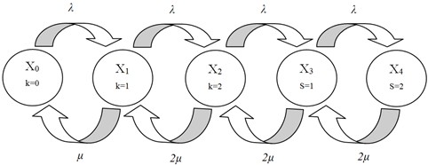
The obtained values of the time points of arrival of cars at the service station are postponed on the graph (Fig. 2).

Next, using Eq. (4), we simulate the time spent on servicing each regular machine. The random numbers $y_{i}$ corresponding to the second row of Table 1 are: 0.51; 0.41; 0.38, etc.

To do this, we first calculate the density or intensity of the service:

μ = \frac{1}{M_{t_{s e r v .}}} = \frac{1}{2.5} = 0.4 .

Now let’s use the Eq. (4):

∆ t_{1}^{* *} = - \frac{1}{μ} ∙ 2.3 l g (1 - y_{1}) = \frac{0.23}{0.4} l g (1 - 0.51) = 5.75 l g 0.49 = - 5.75 (- 0.31) = 1.7825 \approx 1.78 .

Received time values $∆ t_{1}^{* *} = 1.78$ is entered in Table 3. Similarly, we calculate the value of the service time for the remaining machines. Taking into account the time of arrival of the cars and the time spent on their maintenance, we calculate the start and end times of service for each of the cars (Table 3).

Fig. 2A graph for calculating the state time of a queuing system with two channels and two places to wait in a queue (λ= 1.5 cars/hour and Mserv.= 2.5 hours)

Based on the graph, we calculate the frequencies of system states obtained based on a single implementation for a 10-hour working day ( $T_{t o t} =$ 10):

P_{o} = \frac{T_{0}}{Т_{t o t}} = \frac{0.21 + 0.33}{10} = 0.054,

where $P_{o}$ – the probability of complete station downtime) and:

P_{1} = \frac{T_{1}}{T_{t o t}} = \frac{0.95 + 0.07 + 0.31 + 0.78 + 0.24}{10} = \frac{2.35}{10} = 0.235,

P_{2} = \frac{T_{2}}{T_{t o t}} = \frac{0.83 + 0.29 + 0.7 + 0.15 + 0.13 + 0.47}{10} = \frac{2.57}{10} = 0.257,

P_{3} = \frac{T_{3}}{T_{t o t}} = \frac{0.21 + 0.97 + 0.28 + 0.23 + 1.23}{10} = \frac{2.92}{10} = 0.292,

P_{4} = \frac{T_{4}}{Т_{t o t}} = \frac{0.73 + 0.89}{10} = \frac{1.62}{10} = 0.162,

where $P_{4}$ – the probability of a fully loaded station, also known as the probability of failure.

Table 3Calculation of the moments of the beginning and end of car maintenance at the service station

Car number	1	2	3	4	5	6	7	8	9	10	11	12
Random numbers, $y_{i}$	0.51	0.43	0.38	0.54	0.06	0.61	0.52	0.43	0.47	0.72	0.46	0.67
Service time, $∆ t_{1}^{* *}$	1,78	1.4	1.2	1.94	0.15	2.35	1.83	1.4	1.59	3.18	1.54	2.77
Start of service, $t_{i . s t a r t}^{* *}$	0.21	1.16	2.06	2.56	3.57	4.83	5.07	6.9	7.18	8.3	8.77	Refusal issued
End of service $t_{i . e n d}^{* *}$	1.99	2.56	3.26	4.5	3.72	7.18	6.9	8.3	8.77	11.48	10.31	Refusal issued

We check the correctness of the calculations performed:

\sum_{i = 1}^{n} P_{i} = (0.054 + 0.235 + 0.257 + 0.292 + 0.162) = 1 .

We determine the probability of system failure. Of the total number of cars arriving at the station during the 10-hour working day (13 cars), the 12th and 13th were refused. Therefore, the probability of failure is [11]:

P_{f a i l .} = \frac{2}{13} = 0.154 .

Calculating the average number of busy channels:

M [k] = \sum_{k = 0}^{n} k P_{k} + n \sum_{s = 1}^{m} P_{n + s} = 1 ∙ P_{1} + 2 ∙ P_{2} + 2 ∙ (P_{3} + P_{4})

= 1 ∙ 0.235 + 2 ∙ 0.257 + 2 ∙ (0.292 + 0.162) = 1.657,

M [s] = \sum_{s = 1}^{m = 2} s ∙ P_{n + s} = 1 ∙ P_{3} + 2 ∙ P_{4} = 1 ∙ 0.292 + 2 ∙ 0.162 = 0.616 .

We calculate the average waiting time in the queue for cars located in the waiting room:

t_{a v e r . t i m e} = \frac{T_{3} + 2 T_{4}}{N - N_{f a i l .}} = \frac{2.92 + 2 ∙ 1.62}{13 - 2} = 0.56 h o u r s .

We determine the total average time spent by the application in the system:

t_{t o t .} = t_{a v e r . t i m e} + M_{t_{s e r v .}} = 0.56 + 2.5 = 3.06 h o u r s .

It should be noted that the obtained characteristics correspond to one implementation of the process, i.e. correspond to one working day of operation of the station. To obtain more accurate results, depending on the required accuracy, the number of implementations should be increased to 100-1000 implementations. Then, averaging the obtained frequencies $P_{0}^{*}$ , $P_{1}^{*}$ ,…, $P_{4}^{*}$ , more accurate values of the mathematical expectation of the number of occupied channels, the mathematical expectation of the queue length and other characteristics are obtained.

4. Discussions

The results obtained during the application of the statistical modeling method to analyze the operation of a car service station demonstrate the high effectiveness of this approach in solving the problems of queuing theory. The method made it possible to accurately calculate the numerical characteristics of the system's functioning, such as the probability of states, the average number of busy channels, the waiting time in the queue, and the average time an application stays in the system [12].

One of the main conclusions of the study is that statistical modeling makes it possible to identify not only general trends in the system, but also potential problems, such as a high probability of failure, which can significantly affect the system’s throughput. In the studied model for a car service station, the probability of failure was 15.4 %, which indicates possible capacity problems with an increase in the number of requests, especially in conditions of a limited number of service channels and waiting areas.

In addition, the results obtained confirm that in order to obtain more accurate characteristics of the system, it is necessary to carry out several modeling implementations. In this case, the study was based on a single process implementation, which yielded average results for one working day [13]. However, in order to increase the accuracy of calculations and obtain more reliable statistical estimates, it is necessary to increase the number of implementations to 1000 or more, which will reduce errors and provide more reliable conclusions about the functioning of the system in real conditions.

The statistical modeling method has also demonstrated its versatility. It can be used not only to solve problems in queuing theory, but also for other areas such as assessing the reliability of technical systems, calculating the capacity of transport interchanges, determining the optimal number of spare parts for maintaining transport and tractor fleets, and analyzing other complex logistics processes. This opens up prospects for a wide application of the method in various fields related to transport and maintenance.

Thus, the results of the study confirm the importance of statistical modeling as a powerful tool for optimizing the operation of transport systems, increasing their efficiency and reliability.

5. Conclusions

According to the stated purpose of the article, the effectiveness of the statistical modeling method was proved using the example of using random numbers. The results of this study will be the initial stage as a method for determining the traffic flow and allows for further research based on experimental data.

In conclusion, we note that the statistical modeling method can be used not only to solve problems in queuing theory, but also for other tasks, for example: 1) to determine the reliability of complex technical systems; 2) to determine the capacity of transport and logistics centers, specialized international customs control posts; 3) to determine the optimal number of spare parts, components and assemblies necessary to maintain a given automotive and tractor fleet in good condition; 4) to determine the capacity of highways, transport interchanges and for solving other tasks.

Thus, a well-founded statistical modeling method covers both operational management tasks and strategic planning, which provides an opportunity for further research, taking into account the results of experimental and field studies at the landfill.

References

A. Terentyev, M. Karelina, V. Egorov, A. Andreev, and K. Reza Kashyzadeh, “Model for determining optimal routes in complex transport systems,” Transportation Research Procedia, Vol. 57, pp. 679–687, Jan. 2021, https://doi.org/10.1016/j.trpro.2021.09.100

Publisher
S. A. Evtiukov, E. V. Kurakina, and S. S. Evtiukov, “Smart transport in road transport infrastructure,” in IOP Conference Series: Materials Science and Engineering, Vol. 832, No. 1, p. 012094, Apr. 2020, https://doi.org/10.1088/1757-899x/832/1/012094

Publisher
I. Chernyaev, E. Oleshchenko, and I. Danilov, “Methods for continuous monitoring of compliance of vehicles’ technical condition with safety requirements during operation,” Transportation Research Procedia, Vol. 50, pp. 77–85, Jan. 2020, https://doi.org/10.1016/j.trpro.2020.10.010

Publisher
M. O. Mussabekov, G. B. Bakyt, A. M. Omirbek, E. Brumerčíková, and B. Buková, “Shunting locomotives fuel and power resources decrease,” in MATEC Web of Conferences, Vol. 134, p. 00041, Nov. 2017, https://doi.org/10.1051/matecconf/201713400041

Publisher
C. Sommer, “Shortest-path queries in static networks,” ACM Computing Surveys, Vol. 46, No. 4, pp. 1–31, Mar. 2014, https://doi.org/10.1145/2530531

Publisher
K. Zhussupov, A. Toktamyssova, S. Abdullayev, G. Bakyt, and M. Yessengaliyev, “Investigation of the stress-strain state of a wheel flange of the locomotive by the method of finite element modeling,” Mechanics, Vol. 24, No. 2, pp. 174–181, May 2018, https://doi.org/10.5755/j01.mech.24.2.17637

Publisher
L. Vukić, T. Poletan Jugović, G. Guidi, and R. Oblak, “Model of determining the optimal, green transport route among alternatives: data envelopment analysis settings,” Journal of Marine Science and Engineering, Vol. 8, No. 10, p. 735, Sep. 2020, https://doi.org/10.3390/jmse8100735

Publisher
G. Bakyt, Y. Jailaubekov, S. Abdullayev, G. Ashirbayev, and I. Ashirbayeva, “Assessment of carbon dioxide emissions in road transport, using exhaust gas cleaning technology, in the Republic of Kazakhstan,” Vibroengineering Procedia, Vol. 48, pp. 87–92, Feb. 2023, https://doi.org/10.21595/vp.2023.23163

Publisher
S. Abdullayev, G. Imasheva, N. Tomkurzina, N. Adilova, and G. Bakyt, “Prospects for the use of gondola cars on bogies of model ZK1 in the organization of heavy freight traffic in the Republic of Kazakhstan,” Mechanics, Vol. 24, No. 1, pp. 32–36, Feb. 2018, https://doi.org/10.5755/j01.mech.24.1.17710

Publisher
D. Rabar, “An overview of data envelopment analysis application in studies on the socio-economic performance of OECD countries,” Economic Research-Ekonomska Istraživanja, Vol. 30, No. 1, pp. 1770–1784, Oct. 2017, https://doi.org/10.1080/1331677x.2017.1383178

Publisher
S. Abdullayev, N. Tokmurzina, and G. Bakyt, “The determination of admissible speed of locomotives on the railway tracks of the Republic of Kazakhstan,” Transport Problems, Vol. 11, No. 1, pp. 61–68, Jan. 2016, https://doi.org/10.20858/tp.2016.11.1.6

Publisher
S. Soheilirad, K. Govindan, A. Mardani, E. K. Zavadskas, M. Nilashi, and N. Zakuan, “Application of data envelopment analysis models in supply chain management: a systematic review and meta-analysis,” Annals of Operations Research, Vol. 271, No. 2, pp. 915–969, Sep. 2017, https://doi.org/10.1007/s10479-017-2605-1

Publisher

About this article

Received

18 April 2025

Accepted

03 May 2025

Published

15 May 2025

SUBJECTS

Mathematical models in engineering

DOI

https://doi.org/10.21595/vp.2025.25012

Keywords

statistical modelling

mass service theory

mathematical expectation

probabilistic models

mass service system

random numbers

service stations

Acknowledgements

The authors have not disclosed any funding.

Data Availability

The datasets generated during and/or analyzed during the current study are available from the corresponding author on reasonable request.

Conflict of interest

The authors declare that they have no conflict of interest.

This is an open access article distributed under the Creative Commons Attribution License, which permits unrestricted use, distribution, and reproduction in any medium, provided the original work is properly cited.

Previous article in issue Previous Next article in issue Next

A. Tulenov, Y. Baubekov, B. Shoibekov, G. Bakyt, G. Bekbolatov, and O. Ablyalimov, “Application of statistical modelling method for determination of optimal solutions of road transport problems,” Vibroengineering Procedia, Vol. 58, pp. 387–394, May 2025, https://doi.org/10.21595/vp.2025.25012

Copy Extrica

Copied to clipboard!

TY  - JOUR
DO  - 10.21595/vp.2025.25012
UR  - https://doi.org/10.21595/vp.2025.25012
TI  - Application of statistical modelling method for determination of optimal solutions of road transport problems
T2  - Vibroengineering Procedia
AU  - Tulenov, Aidarali
AU  - Baubekov, Yermek
AU  - Shoibekov, Baurzhan
AU  - Bakyt, Gabit
AU  - Bekbolatov, Gabit
AU  - Ablyalimov, Oleg
PY  - 2025
DA  - 2025/05/15
PB  - Extrica
SP  - 387-394
VL  - 58
SN  - 2345-0533
SN  - 2538-8479
ER  - 

Copy Ris

Copied to clipboard!

 @article{Tulenov_2025, title={Application of statistical modelling method for determination of optimal solutions of road transport problems}, volume={58}, ISSN={2538-8479}, url={https://doi.org/10.21595/vp.2025.25012}, DOI={10.21595/vp.2025.25012}, journal={Vibroengineering Procedia}, publisher={JVE International Ltd.}, author={Tulenov, Aidarali and Baubekov, Yermek and Shoibekov, Baurzhan and Bakyt, Gabit and Bekbolatov, Gabit and Ablyalimov, Oleg}, year={2025}, month=may, pages={387–394} }

Copy Bibtex

Copied to clipboard!

[1]A. Tulenov, Y. Baubekov, B. Shoibekov, G. Bakyt, G. Bekbolatov, and O. Ablyalimov, “Application of statistical modelling method for determination of optimal solutions of road transport problems,” Vibroengineering Procedia, vol. 58, pp. 387–394, May 2025, doi: 10.21595/vp.2025.25012.

Copy IEEE

Copied to clipboard!

Tulenov, Aidarali, Yermek Baubekov, Baurzhan Shoibekov, Gabit Bakyt, Gabit Bekbolatov, and Oleg Ablyalimov. “Application of Statistical Modelling Method for Determination of Optimal Solutions of Road Transport Problems.” Vibroengineering Procedia 58 (May 15, 2025): 387–94. https://doi.org/10.21595/vp.2025.25012.

Copy Chicago

Copied to clipboard!

27	76	74	35	84	85	30	18	89	77	29	49	06	97	14
03	54	51	43	38	54	06	61	52	43	47	72	46	67	33
80	21	73	62	92	98	52	52	43	35	24	43	22	48	96
10	87	56	20	04	90	30	16	11	05	57	41	10	63	68
54	12	75	73	26	26	62	91	90	87	24	47	28	87	78

27	76	74	35	84	85	30	18	89	77	29	49	06	97	14
03	54	51	43	38	54	06	61	52	43	47	72	46	67	33
80	21	73	62	92	98	52	52	43	35	24	43	22	48	96
10	87	56	20	04	90	30	16	11	05	57	41	10	63	68
54	12	75	73	26	26	62	91	90	87	24	47	28	87	78

Application of statistical modelling method for determination of optimal solutions of road transport problems

Abstract

Highlights

1. Introduction

2. Materials and methods

3. Results

4. Discussions

5. Conclusions

References

About this article

Related Articles

27	76	74	35	84	85	30	18	89	77	29	49	06	97	14
03	54	51	43	38	54	06	61	52	43	47	72	46	67	33
80	21	73	62	92	98	52	52	43	35	24	43	22	48	96
10	87	56	20	04	90	30	16	11	05	57	41	10	63	68
54	12	75	73	26	26	62	91	90	87	24	47	28	87	78