Abstract
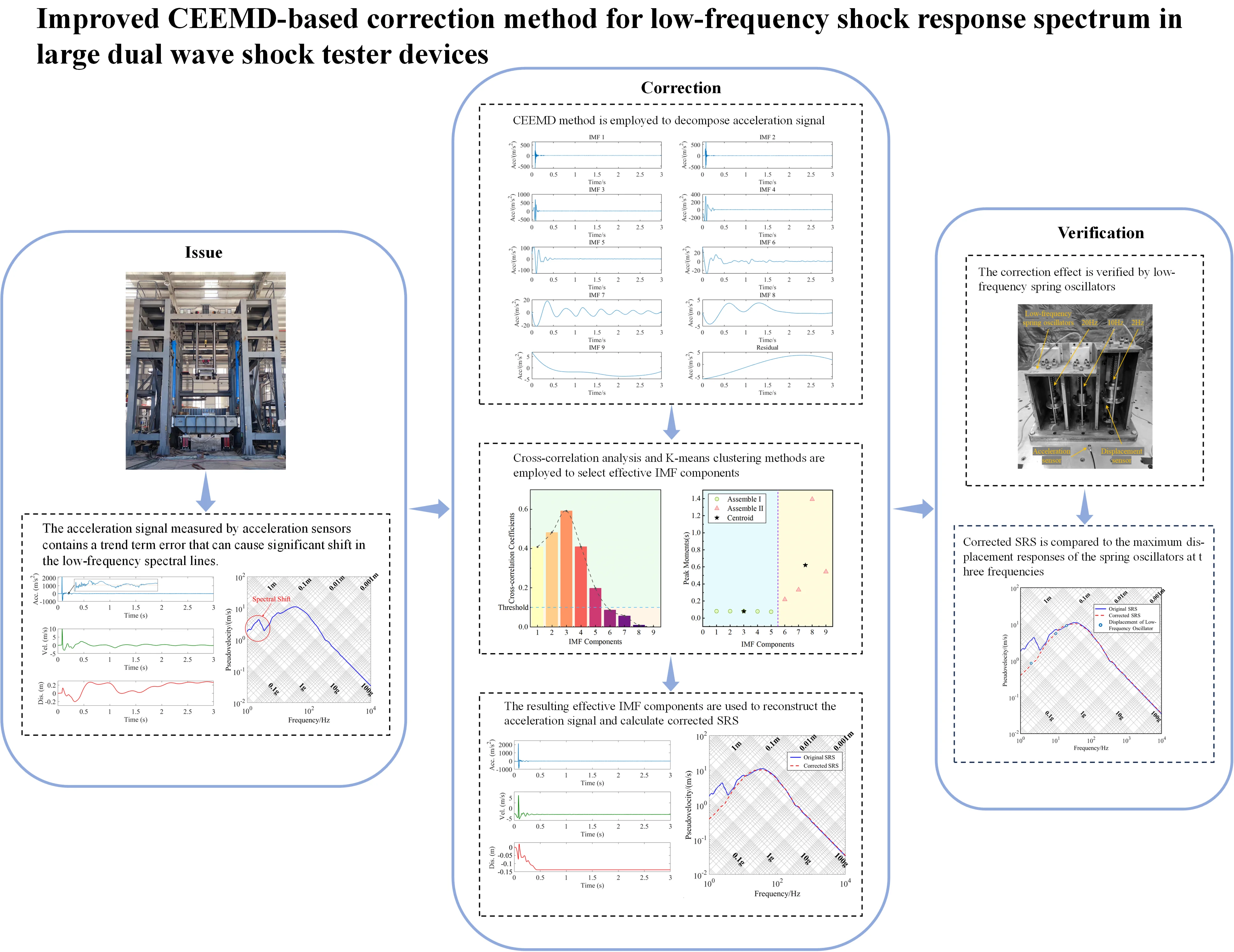
The shock response spectrum (SRS), calculated from a shock acceleration signal, is a critical indicator of shock environments. However, under intense loads, acceleration sensors are prone to trend term errors that can cause significant drift in the low-frequency spectral lines of large dual-wave shock tester devices. To address this issue, the complementary ensemble empirical mode decomposition (CEEMD) method was employed to decompose acceleration signals and restore the actual shock environment. Intrinsic mode functions (IMFs) were cross-correlated and compared to a predefined threshold to identify the effective IMF components required to reconstruct the signal. K-means clustering was employed to further validate the effectiveness of the IMFs for enhanced selection accuracy. Finally, the reconstructed acceleration signal was used to calculate a corrected SRS. The proposed approach demonstrated significant improvements over the traditional CEEMD algorithm. The corrected SRS exhibits a 5.6316 dB/oct slope in the low-frequency band, reflecting an equal displacement trend. The maximum error at the corresponding frequency was less than 6 % in comparison to the relative displacement response measured by low-frequency spring oscillators. This improved CEEMD correction method can effectively restore the actual shock environment of a dual-wave shock tester device, offering a valuable reference for evaluating shock resistance in onboard equipment.
Highlights
- An improved CEEMD method was used to remove the trend term error of acceleration during the large dual-wave shock test.
- We combined cross-correlation analysis and K-means clustering to select the effective IMF components and reconstruct the acceleration signal.
- Low-frequency spring oscillators that we developed were employed to verify the accuracy of shock response spectrum correction results.
- The correction method proposed in this paper can effectively restore the actual shock environment of a dual-wave shock tester device, offering a valuable reference for evaluating shock resistance in onboard equipment.
1. Introduction
Rapid advancements in weaponry place ships under increasing threats from underwater weapons, with underwater explosions as the most common method of attack [1]. These explosions generate two primary shock effects: shock waves and bubble pulsations [2]. Shock waves, characterized by high frequency and large peak values, propagate rapidly and can directly damage local structures on ships and equipment. In contrast, bubble pulsations have lower frequency but higher energy; they propagate more slowly but can significantly impact overall structural integrity [3]. Therefore, rigorous shock testing is essential for critical onboard equipment.
Whole-ship or floating shock platform explosion tests are effective. However, they are also expensive, time-consuming, and dangerous [4]. As an alternative, shock tester devices that partially simulate positive and negative dual-wave effects of underwater explosions have become vital for evaluating the shock resistance of medium and small-sized onboard equipment [5-6]. The shock response spectrum (SRS) is a curve that represents the maximum response of a single-degree-of-freedom (SDOF) system to shock loads as a function of natural frequency, serving as a critical metric for the explosion shock environment [7-10].
Accurate shock environment representation is essential for obtaining reliable evaluation results. However, during testing, the physical structure of acceleration sensors can lead to resonance peaks under strong shock loading; this prevents the immediate release of generated charges, causing the measured acceleration signal to include trend term errors [11, 12]. These errors result in significant spectral line drift in the low-frequency band of the calculated SRS. Therefore, correcting the measured acceleration signal is necessary to reproduce the actual shock environment.
Several methods are currently used to address trend term errors in shock acceleration signals, including high-pass filtering [13], least squares fitting [14], wavelet transform [15-17], and empirical mode decomposition (EMD) [18-20]. He. et al. [21] employed high-pass filtering to a signal, with frequency-domain differentiation for signal processing, to analyze and process multi-source vibration signals via wavelet decomposition and reconstruction techniques. They effectively filtered out low-frequency trend components by setting an appropriate cutoff frequency. V. J. Grillo et al. [22] employed least squares fitting to integrate velocity and eliminate trend components, followed by differentiation, to obtain corrected acceleration data. El Ghazouly et al. [23] employed wavelets as a de-trending tool. They conducted a detailed analysis to identify the optimal wavelet base function and threshold technique estimator by comparing different wavelet parameters. using different thresholding techniques to significantly reduce the double difference error. M. F. Kaleem et al. [24] empirically analyzed non-stationary signals in the context of de-noising, de-trending, and discrimination applications. They innovatively modified the EMD algorithm for time-scale-based signal decomposition, then employed hierarchical decomposition to divide a signal into selected frequency bands, effectively removing trend term errors.
Complete ensemble empirical mode decomposition (CEEMD), an extension of ensemble empirical mode decomposition (EEMD), addresses the issue of residual white noise in the EEMD method that persists after averaging and cannot be fully offset [25]. CEEMD uses equal-amplitude inverse noise to eliminate residual auxiliary noise in the reconstructed signal. This approach significantly reduces the number of noise ensembles compared to EEMD, enhancing computational efficiency while preventing mode mixing, eliminating noise effects, and stabilizing the decomposition. These advantages allow CEEMD to handle complex, nonlinear, and non-stationary signals more effectively [26]-[27].
Li et al. [28] employed a time and frequency analysis method based on the CEEMD algorithm to correct ground-penetrating radar signals. They extracted time- and frequency-domain signals from each IMF component and compared the results of their method with the Hilbert-Huang transform. However, their analysis primarily evaluated the time-domain features of each IMF without considering the relationship between the IM components and the original signal in terms of content. This limitation highlights the need for an SRS correction method based on CEEMD that can filter IMF components based on content and evaluate their time-domain characteristics to effectively remove trend term errors.
This study employs the CEEMD algorithm to decompose an acceleration signal into several IMF components. Cross-correlation analysis is performed each IMF component to calculate the correlation coefficient, which is compared against a predefined threshold to identify effective IMFs. The peak moments of these components are extracted, then K-means clustering is applied to classify and further assess their validity. The proposed method is validated by comparison with other correction algorithms and the measured displacement response of low-frequency spring oscillators.
The remainder of this paper is organized as follows: Section 2 introduces the principles underlying the SRS correction methodology, including SRS calculation, the CEEMD algorithm, cross-correlation analysis, and K-means clustering. Section 3 outlines the SRS correction process. Section 4 compares the correction effects of various decomposition algorithms and validates the correction through low-frequency spring oscillator tests. Section 5 provides concluding remarks.
2. Principles of SRS correction
2.1. SRS calculation
The SRS, which represents the maximum response values of a series of SDOF systems under a specific shock load as a function of the system’s natural frequency, is widely used in shock-related research [29].
Fig. 1SDOF systems

If a specific shock load is applied to the SDOF, as shown in Fig. 1, then the system’s mathematical model can be described by the following second-order differential equation:
where , , and represent the mass, damping coefficient, and stiffness of the SDOF system, respectively; represents the input shock excitation acceleration signal, and represents the response of the system to the shock signal.
The following can be derived from Eq. (1) by defining the relative displacement of the mass to the base as :
The undamped intrinsic frequency is:
where is the intrinsic frequency in rad/s. The system damping ratio is:
Importantly, is commonly represented by the amplification factor , where is referred to as the “quality factor”.
Substituting Eq. (3) and (4) into Eq. (2) yields the equation of motion for the relative response:
Solving the differential Eq. (5) yields the relationship between the shock response’s peak and the SDOF system’s natural frequency, enabling conversion of the time-domain shock acceleration signal into a frequency-domain SRS.
2.2. Principles of CEEMD algorithm
The CEEMD algorithm enhances EEMD by “completely” ensembling white noise to more accurately mitigate the impact of noise on decomposition results. By adding a pair of auxiliary white noise signals with opposite signs to the signal and averaging the noise to nearly zero, CEEMD effectively avoids the mode-mixing problem of EEMD and achieves higher decomposition accuracy [30].
Assuming is the signal to be decomposed, with a length of , the CEEMD decomposition process unfolds as follows.
(1) Determine the number of iterations, then add a pair of white noise sequences with equal amplitude and opposite signs, and , to the original signal . This generates two sets of noise-contaminated signals, and :
(2) Decompose with CEEMD to obtain two sets of IMF components, and . Here, represents the ensemble mean of the IMFs after adding positive noise; represents the ensemble mean of the IMFs after adding negative noise.
(3) Calculate the mean values of and to determine :
(4) Obtain the mean values for all components after decompositions to determine the final decomposition result.
(5) Decompose the signal into all IMF components and the residual, which represents the non-decomposable trend components of the signal.
The final decomposition results consist of all IMF components and the residual. The IMF components represent the signal’s different frequency or scale components, while the residual corresponds to the low-frequency trend or non-periodic elements of the signal.
2.3. Principles of cross-correlation analysis
This study employs cross-correlation analysis as a critical criterion for selecting effective IMF components. Cross-correlation analysis is a method used to measure the similarity between two sets of signals [31-33]. It is commonly applied in signal processing, image analysis, and time series analysis to detect similarities, time lags, and signal alignments, among other tasks.
The cross-correlation function of two signals and is defined as follows:
where represents the delay time, indicating the time shift of one signal relative to the other.
The cross-correlation coefficient, obtained by normalizing the cross-correlation function, provides a convenient way to compare the similarity between two signals. Assuming two discrete signals and , each of length , the calculation process for the cross-correlation coefficient unfolds over five steps.
(1) Calculate the mean value. First, compute the mean values of signals and :
(2) Remove the mean value. Subtract the mean value of each signal from the signal itself to obtain a signal with a 0 mean:
(3) Calculate the cross-correlation value. For any time delay , the unnormalized value of cross-correlation is:
This represents the correlation between signal and signal at time delay .
(4) Calculate auto-correlation values. The auto-correlation values, defined as:
are employed to normalize the cross-correlation values to a range between [–1, 1].
(5) Calculate the normalized cross-correlation coefficient:
where the cross-correlation coefficient falls within the range [−1, 1]. A value of closer to 1 indicates a higher degree of correlation between the two signals, while a value closer to 0 indicates a lower degree of correlation. After a series of comparative tests, a cross-correlation coefficient threshold of 0.1 is appropriate for selecting effective IMF components.
2.4. Principles of K-means clustering
K-means clustering is employed to further validate the rationality of the selected IMF components. This method groups data based on distance, initially by randomly selecting points as cluster centers, then assigning each data point to the nearest such center to form clusters. After assignment, the cluster centers are recalculated based on the current data points. This iterative process continues until one of the following termination criteria is met: no data points are reassigned, the cluster centers no longer change, or the sum of squared errors reaches a local minimum [34].
The specific steps of K-means clustering are as follows:
(1) Normalize data points and filter out outliers.
(2) Select initial center points, denoted as .
(3) Define the loss function as:
where represents the -th data point, denotes the cluster assigned to , is the center point of the corresponding cluster, and is the total number of data points.
(4) Let represent the iteration step. During the -th iteration, is the cluster assigned to the -th point, and represents the center points. Assign each data point to the nearest center point:
Recalculate the center points to minimize the loss function, and repeat these steps until a termination criterion is met.
3. Correction of SRS for dual-wave shock tester device
3.1. Shock environment measurement process
As shown in Fig. 2, this study employs a 12-t vertical dual-wave shock tester device developed by our institute. The improved CEEMD method eliminates trend term errors in acceleration signals, thereby restoring the actual SRS.
Fig. 2Vertical dual-wave shock tester device
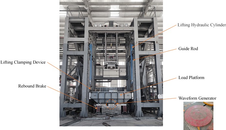
During shock testing, the load platform is lifted to a preset height along the guide rod using the control system. Once the lifting clamping device is released, the platform slides down along the guide rods under the influence of gravity, impacting the waveform generator and producing a positive half-sine acceleration shock wave. Following the shock, a hydraulic damping cylinder buffers and restricts the platform’s motion as it rebounds upward. This creates a negative half-sine shock wave. The full sequence ultimately forms a dual-wave acceleration waveform.
A piezoelectric acceleration sensor is used to measure the shock load during testing. The sensor has a frequency response range of 0.1 Hz-12,600 Hz, a sensitivity of 1 pC/ms2, and a maximum measurement range of 60,000 ms-2. It is configured with a sampling frequency of 1280 Hz and mounted on the surface of the loading platform using a mechanical filter.
3.2. Analysis of original SRS
Shock tests were conducted under four different conditions using the dual-wave shock tester device. For all conditions (I-IV), the acceleration peaked at approximately 0.08 s with maximum values of 2149.1 m/s2, 2491.7 m/s2, 2438.5 m/s2, and 2374.4 m/s2, respectively. Taking Condition I as an example, Fig. 3 shows the acceleration signal and its time-domain integral curve. The acceleration signal does not immediately return to zero after the shock ends but continues to oscillate for some time. Consequently, the integrated velocity derived from the acceleration is non-zero; the integrated displacement increases over time, with the curve exhibiting significant drift. This indicates that the acceleration signal is affected by the trend term error.
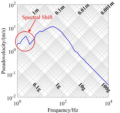
The SRS of the acceleration signal containing trend term error under Condition I was calculated using the method described in Section 2.1, as shown in Fig. 4. According to our references [35], the standard slope of the low-frequency band in the four-coordinate pseudo-velocity shock spectrum is 6 dB/oct. However, the trend term error in the original acceleration signal causes a drift in the low-frequency band of the spectrum, resulting in a slope of –4.878 dB/oct, much smaller than the standard 6 dB/oct.
Using this SRS as the baseline for shock resistance testing would severely compromise the evaluation of low-frequency shipborne equipment. Therefore, removing the trend term error from the acceleration signal is essential before calculating the SRS to accurately reflect the actual shock environment.
Fig. 3Original acceleration signal and its integrated velocity and integrated displacement

a) Acceleration signal

b) Integral velocity

c) Integral displacement
Fig. 4SRS calculated from original acceleration signal
3.3. Correcting SRS based on improved CEEMD
3.3.1. Acceleration signal decomposition
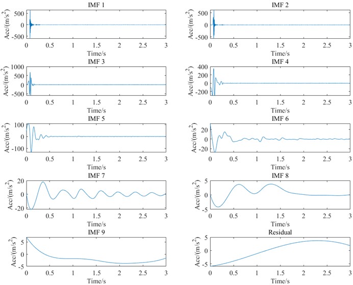
The CEEMD algorithm was employed to decompose the acceleration signal obtained from the dual-wave shock tester device with 10 as the maximum number of iterations, a white noise coefficient of 0.2, and the number of added noises set to 100 [36].
Fig. 5 shows all IMF components and the residual obtained from CEEMD decomposition of the acceleration signal under Condition I. The time scales within each IMF component are consistent, which effectively resolves the mode-mixing problem encountered during EMD decomposition. Thus, the CEEMD algorithm allows for a more accurate decomposition of the shock acceleration signal into its effective IMF components, representing the actual acceleration and ensuring that error components are associated with the trend term.
Fig. 5CEEMD decomposition results of acceleration signal for Con. I
3.3.2. Effective IMF component selection
3.3.2.1. Selection criterion for cross-correlation analysis
Table 1 lists the cross-correlation coefficients of each IMF component under all four conditions. IMF components with cross-correlation coefficients exceeding the threshold were retained as effective components, while those below the threshold were identified as trend term error components and removed. Fig. 6 illustrates the variations in cross-correlation coefficients for each IMF component under Condition I. The first five IMF components have cross-correlation coefficients exceeding the threshold of 0.1, qualifying them as effective IMF components.
Based on the information shown Table 1 and Fig. 6, under Condition I, the first five IMF components are effective and primarily represent the actual acceleration signal. Starting from the 6th IMF component, the cross-correlation coefficients all fall below 0.1 and gradually approach zero, indicating that they are dominated by trend term error.
However, cross-correlation analysis is sensitive to noise. When the signal contains significant noise, some effective IMFs may exhibit high correlations with the noise components, resulting in their misclassification as trend components. In such cases, relying solely on cross-correlation analysis to select effective IMFs may lead to unreliable results. Therefore, it is essential to evaluate each IMF more comprehensively by considering both its spectral and temporal characteristics.
Fig. 6Cross-correlation coefficients of each IMF for Con. I
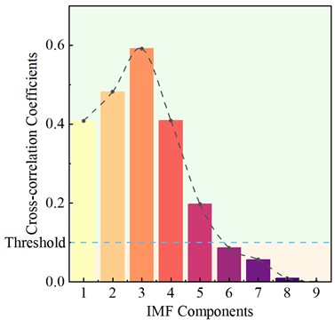
Table 1Cross-correlation coefficients of each IMF
Coefficient | |||||||||
Condition | IMF1 | IMF2 | IMF3 | IMF4 | IMF5 | IMF6 | IMF7 | IMF8 | IMF9 |
Con. I | 0.4079 | 0.4817 | 0.5915 | 0.4087 | 0.1973 | 0.0864 | 0.0562 | 0.0091 | –0.0002 |
Con. II | 0.3930 | 0.4458 | 0.7158 | 0.3343 | 0.2046 | 0.0658 | 0.0579 | 0.0175 | 0.0002 |
Con. III | 0.3650 | 0.4883 | 0.5448 | 0.3035 | 0.1407 | 0.0624 | 0.0529 | 0.0013 | –0.0012 |
Con. IV | 0.3817 | 0.4734 | 0.7440 | 0.3330 | 0.2176 | 0.0891 | 0.0582 | 0.0095 | 0.0012 |
3.3.2.2. Selection criterion for K-means clustering
The acceleration signals of the dual-wave shock tester are complex oscillatory signals. The K-means clustering method was employed to prevent over-removal of the effective components selected through cross-correlation coefficients, ensuring reliable results.
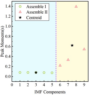
Table 2 lists the peak moments of each IMF component under the four conditions. The peak moments were divided into effective components and trend components based on K-means clustering, with the number of centroids 2. Fig. 7 illustrates the results after applying K-means clustering to divide the peak moments of IMF components. The first five IMF components fall into the first category; the 6th to 9th IMF components comprise the second category. The peak moments of the first five IMF components are nearly identical, concentrated around 0.08 s.
Table 2Peak moments of each IMF
Peak moments | |||||||||
Conditions | IMF1 | IMF2 | IMF3 | IMF4 | IMF5 | IMF6 | IMF7 | IMF8 | IMF9 |
Con. I | 0.080 | 0.080 | 0.080 | 0.078 | 0.075 | 0.2175 | 0.331 | 1.393 | 0.544 |
Con. II | 0.081 | 0.080 | 0.080 | 0.079 | 0.077 | 0.2653 | 0.320 | 1.352 | 2.065 |
Con. III | 0.081 | 0.080 | 0.080 | 0.076 | 0.075 | 0.3114 | 0.383 | 0.599 | 1.106 |
Con. IV | 0.081 | 0.080 | 0.080 | 0.079 | 0.069 | 0.2366 | 0.360 | 0.7083 | 1.593 |
As shown in Table 2 and Fig. 7, the first five IMF components were identified as the primary constituents of the actual acceleration signal. The peak moments show significant deviations from the 6th IMF component onward, indicating that these components are dominated by trend term errors. By combining the results of cross-correlation analysis and K-means clustering, the 6th to 9th IMF components and the residual can be identified as trend term errors caused by the measurement system and external environmental factors. These components should be excluded during the reconstruction of the acceleration signals to ensure accuracy.
Fig. 7K-means clustering division results at the peak moments of each IMF for Con. I
3.3.3. Reconstruction of acceleration signals and analysis of corrected SRS
Based on the filtered results reported the previous section, IMF1 to IMF5 were selected to reconstruct the acceleration signal. Fig. 8 shows the corrected acceleration signal and its time-domain integration curve for Condition I. After reconstruction, the acceleration signal rapidly returns to zero following the shock and oscillations are eliminated. The integral velocity approaches zero, and the displacement curve stabilizes after the shock ends. These results demonstrate that the CEEMD decomposition of the original acceleration signal, combined with cross-correlation analysis and K-means clustering, successfully reveals effective IMF components to produce a reconstructed acceleration signal free from trend term error interference.
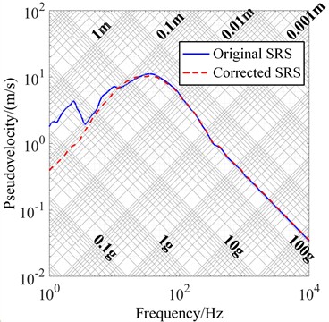
According to Eqs. (3)-(5), the reconstructed acceleration signal was employed to calculate the SRS. Fig. 9 shows a comparison of the SRS before and after this correction under Condition I. The corrected low-frequency spectral slope is 5.6316 dB/oct, with a 6.14 % error relative to the standard slope; the SRS exhibits an equal displacement trend in the 4-20 Hz range.
4. Verification of correction effect for low-frequency SRS
4.1. Correction effects of different decomposition algorithms
EMD is well-suited for analyzing and processing non-stationary and nonlinear shock signals. However, the mode-mixing effect persists during EMD decomposition, leading to inaccuracies in each IMF component’s frequency distribution. EEMD reduces mode mixing by adding white noise to the original signal before decomposition. However, residual white noise remains after averaging in EEMD and cannot be entirely offset. CEEMD addresses this limitation through further refinement.
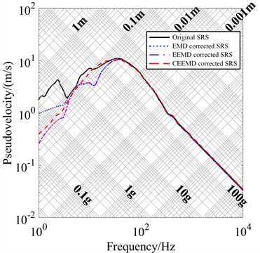
As shown in Fig. 10, under Condition I, EMD, EEMD, and CEEMD were applied to decompose and reconstruct an original acceleration signal to obtain the SRS. The maximum iteration number was set to 10 for both EMD and EEMD, which is consistent with the parameters of the CEEMD algorithm. Cross-correlation analysis and K-means clustering were also employed to select effective IMF components.
Fig. 8Corrected acceleration signal and its integrated velocity and integrated displacement

a) Corrected acceleration signal

b) Integral velocity

c) Integral displacement
Fig. 9SRS before and after correction
Using EMD for decomposition and reconstruction led to an SRS with mode-mixing issues, causing overlap between IMF frequency bands and distortion in the low-frequency region. As the figure also shows, the resulting slope is 2.037 dB/oct and the low-frequency SRS values deviate significantly from the actual values. When EEMD is applied, the decomposition introduces residual white noise with random characteristics that create noticeable fluctuations in the low-frequency SRS.
CEEMD, however, not only mitigates mode mixing but also effectively eliminates the influence of residual noise. Combined with cross-correlation analysis and K-means clustering, it ensures precise decomposition and selection of effective IMF components. The corrected SRS closely aligns with the low-frequency equal displacement characteristics, achieving a slope of 5.731 dB/oct. In practice, this would significantly enhance the accuracy of shock resistance evaluation tests.
The correction results indicate that a method combining CEEMD decomposition, cross-correlation analysis, and K-means clustering effectively removes trend term errors in acceleration signals. This approach accurately reflects actual shock environments and could play a crucial role in improving the precision of onboard equipment shock evaluations.
Fig. 10Comparison of correction effect of different methods for Con. I
4.2. Low-frequency spring oscillators verification tests
Based on the fundamental principles of the SRS outlined in Section 2.1, an SDOF linear sprin-mass system (referred to as “spring oscillators”) was employed during a shock test to measure the maximum displacement responses at three fixed frequencies. These results were compared with the low-frequency SRS obtained after correction to further verify the accuracy of the proposed method [37].
4.2.1. Structure of spring oscillators
The spring oscillator set used in this study consists of double helical compression springs with natural frequencies of 2 Hz, 10 Hz, and 20 Hz. Each spring oscillator exists independently without mutual interference. The three spring oscillators are mounted on the same base to ensure exposure to identical shock loads during testing. The assembly diagram is shown in Fig. 11.
Fig. 11Assembly of low-frequency spring oscillator
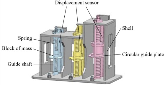
The spring oscillator primarily consists of springs, mass blocks, guiding devices, a shell, and connectors. The springs serve as the core component, providing elastic restoring force. Two pre-compressed springs were used due to the non-linear characteristics of compression springs under tension. The guiding devices ensure that the mass block vibrates in a specified direction, preventing unnecessary displacement or rotation while offering anti-friction and dust-proof functions. Spring seats integrated into the mass blocks and shell position the springs securely.
A magnetostrictive non-contact displacement sensor was employed to record the displacement of mass blocks in the low-frequency oscillator. The sensor has a sensitivity of 100 mV/mm and a range of 200 mm. Compared to contact-type sensors, it reduces damping in the low-frequency oscillator and improves measurement accuracy. Calibration revealed that the actual natural frequencies of the three low-frequency oscillators were 1.937 Hz, 9.687 Hz, and 19.37 Hz, with deviations from the design frequencies of 3.15 %, 3.13 %, and 3.15 %, respectively. The damping ratios were only 0.0371, 0.0145, and 0.0111, while the displacement measurement accuracies were 98.89 %, 96.72 %, and 96.48 %. These results indicate that the low-frequency oscillator set is highly precise and has low damping ratios, making it suitable for accurate measurement in low-frequency shock environments.
4.2.2. Experimental validation results
During the experiment, the low-frequency spring oscillator set was rigidly connected to the shock table surface with bolts. The set was mounted adjacent to the acceleration sensor to ensure consistency with the sensor’s measurements, as shown in Fig. 12. Table 3 presents the maximum displacement responses of the oscillator set under Conditions I-IV.
Fig. 12Shock test site layout
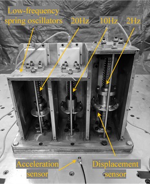
Table 3Maximum displacement response of low-frequency spring oscillator
Conditions | 2 Hz | 10 Hz | 20 Hz |
Con. I | 51.42 mm | 49.60 mm | 50.38 mm |
Con. II | 58.56 mm | 61.42 mm | 57.78 mm |
Con. III | 30.94 mm | 28.74 mm | 30.55 mm |
Con. IV | 57.66 mm | 60.13 mm | 58.62 mm |
Again, taking Condition I as an example, the low-frequency spectral lines of the corrected SRS were compared to the maximum displacement responses of the spring oscillator at three frequencies. This visual comparison highlights the effectiveness of the correction applied to the low-frequency SRS of the dual-wave shock tester.
Fig. 13 shows the measured displacement responses of the low-frequency spring oscillator set compared to the corrected low-frequency SRS spectral line. The errors at the three frequencies are 3.09%, 5.06%, and 3.94%. The slope of the corrected low-frequency spectral line is 5.6316 dB/oct, which falls within a reasonable range. These results demonstrate that the proposed method effectively eliminates trend term errors in acceleration signals and accurately reflects the actual shock environment.
Fig. 13Measured displacement of spring oscillator versus position of SRS
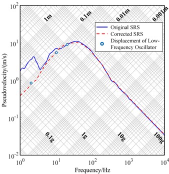
Fig. 14Correction results of SRS for Con. II to Con. IV
a) Condition II
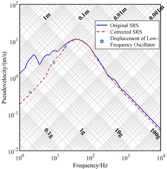
b) Condition III
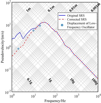
c) Condition IV
Table 4Correction errors for four conditions
Conditions | 2 Hz | 10 Hz | 20 Hz |
Con. I | 3.09 % | 5.06 % | 3.94 % |
Con. II | 5.03 % | 4.72 % | 2.31 % |
Con. III | 8.45 % | 6.34 % | 6.17 % |
Con. IV | 5.82 % | 4.36 % | 6.24 % |
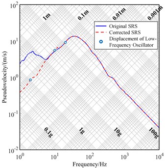
Corrected SRS curves under Conditions II-IV were obtained using the proposed method as shown in Fig. 14. The slopes of the low-frequency spectral lines improved from –6.041 dB/oct, –12.912 dB/oct, and –12.873 dB/oct to 5.535 dB/oct, 5.672 dB/oct, and 5.604 dB/oct after the correction. Table 4 presents the correction results for the low-frequency SRS under all four conditions, comparing them with the measured displacement responses of the low-frequency spring oscillator at the same three frequencies. The maximum errors are 5.06 %, 5.03 %, 8.45 %, and 6.24 %.
These findings indicate that the improved CEEMD method proposed in this paper effectively eliminates trend term errors in acceleration signals, reflects the actual shock environment accurately, and significantly enhances the effectiveness of shock resistance evaluations for onboard equipment.
5. Conclusions
1) The low-frequency band of acceleration signals obtained from large-scale dual-wave shock tester devices contains trend term errors, causing spectral line drift in the calculated SRS. Correcting the low-frequency spectral line is essential to eliminate these errors and accurately restore the actual shock environment.
2) Using the CEEMD method to decompose the acceleration signals and calculate the cross-correlation coefficients for each IMF component allows for accurate classification of IMF components into effective and trend components. K-means clustering can then be employed to classify the peak moments of each component, providing additional validation of the selected effective IMF components’ rationality.
3) Compared to EMD and EEMD algorithms, the proposed improved CEEMD approach effectively suppresses low-frequency spectral line drift in the SRS. The corrected low-frequency spectral line achieves an average slope of 5.658 dB/oct, which satisfies the requirements for shock evaluation.
4) Compared to the measured relative displacement response of a low-frequency spring oscillator, the maximum error of the corrected low-frequency spectral line at corresponding frequencies is 8.45 %. This demonstrates that the proposed method effectively eliminates trend term errors in acceleration signals, providing accurate and reliable shock environment information for evaluating the shock of onboard equipment.
References
-
K. Zhao, D. Shi, Z. Wang, Y. Zhou, and Y. Liang, “Study on critical condition of damage mode of local grillage structure under near-field underwater explosion,” Applied Ocean Research, Vol. 153, p. 104313, Dec. 2024, https://doi.org/10.1016/j.apor.2024.104313
-
F. Mannacio, A. Barbato, F. Di Marzo, M. Gaiotti, C. M. Rizzo, and M. Venturini, “Shock effects of underwater explosion on naval ship foundations: Validation of numerical models by dedicated tests,” Ocean Engineering, Vol. 253, p. 111290, Jun. 2022, https://doi.org/10.1016/j.oceaneng.2022.111290
-
S. Lin, J. Wang, L. Liu, H. Li, T. Ma, and K. Tang, “Research on damage effect of underwater multipoint synchronous explosion shock waves on air-backed clamped circular plate,” Ocean Engineering, Vol. 240, p. 109985, Nov. 2021, https://doi.org/10.1016/j.oceaneng.2021.109985
-
L. Chen, S. Li, Y. Chen, Z. Huan, T. Ai, and Q. Liu, “Damage features and mechanism of prestressed hollow square piles subjected to non-contact underwater explosion,” Structures, Vol. 69, p. 107453, Nov. 2024, https://doi.org/10.1016/j.istruc.2024.107453
-
G. Wang, Y. Xiong, and W. Tang, “A novel heavy-weight shock test machine for simulating underwater explosive shock environment: Mathematical modeling and mechanism analysis,” International Journal of Mechanical Sciences, Vol. 77, pp. 239–248, Dec. 2013, https://doi.org/10.1016/j.ijmecsci.2013.09.006
-
J. Bae, “The Shock-Test Result and Analysis Using Dual-Pulse Shock Testing Machine.,” Journal of the Korea Institute of Military Science and Technology, Vol. 21, No. 3, pp. 342–348, 2018, https://doi.org/10.9766/kimst.2018.21.3.342
-
S. Jayaraman, M. Trikha, Somashekar, D. Kamesh, and M. Ravindra, “Response spectrum analysis of printed circuit boards subjected to shock loads,” Procedia Engineering, Vol. 144, pp. 1469–1476, Jan. 2016, https://doi.org/10.1016/j.proeng.2016.06.710
-
X. Wang, Z. Qin, J. Ding, and F. Chu, “Finite element modeling and pyroshock response analysis of separation nuts,” Aerospace Science and Technology, Vol. 68, pp. 380–390, Sep. 2017, https://doi.org/10.1016/j.ast.2017.05.028
-
W. Sun, Q. Su, H. Yuan, and L. Liu, “Calculation and characteristic analysis on different types of shock response spectrum,” in Journal of Physics: Conference Series, Vol. 1676, No. 1, p. 012236, Nov. 2020, https://doi.org/10.1088/1742-6596/1676/1/012236
-
S. Henclik, “Application of the shock response spectrum method to severity assessment of water hammer loads,” Mechanical Systems and Signal Processing, Vol. 157, p. 107649, Aug. 2021, https://doi.org/10.1016/j.ymssp.2021.107649
-
A. Agnello, “Acceleration sensing technologies for severe mechanical shock,” PCB Piezotronics, Inc., Depew, NY, USA, 2014.
-
W. Babatain, S. Bhattacharjee, A. M. Hussain, and M. M. Hussain, “Acceleration sensors: sensing mechanisms, emerging fabrication strategies, materials, and applications,” ACS Applied Electronic Materials, Vol. 3, No. 2, pp. 504–531, Feb. 2021, https://doi.org/10.1021/acsaelm.0c00746
-
K. R. Sreelekha and T. S. Bindiya, “Design of cost effective variable bandwidth 2D low-pass, high-pass and band-pass filters with improved circularity,” Digital Signal Processing, Vol. 133, p. 103842, Mar. 2023, https://doi.org/10.1016/j.dsp.2022.103842
-
D. Belega and D. Petri, “Effect of windowing and noise on the amplitude and phase estimators returned by the Taylor-based Weighted Least Squares,” Digital Signal Processing, Vol. 83, pp. 202–213, Dec. 2018, https://doi.org/10.1016/j.dsp.2018.09.002
-
Y. Cheng, R. Zhang, and S. Chen, “Wavelet packet transform applied to active noise control system for mixed noise in nonlinear environment,” Digital Signal Processing, Vol. 133, p. 103860, Mar. 2023, https://doi.org/10.1016/j.dsp.2022.103860
-
W. Li, F. Auger, Z. Zhang, and X. Zhu, “Self-matched extracting wavelet transform and signal reconstruction,” Digital Signal Processing, Vol. 128, p. 103602, Aug. 2022, https://doi.org/10.1016/j.dsp.2022.103602
-
Y. Hu, F. Li, H. Li, and C. Liu, “An enhanced empirical wavelet transform for noisy and non-stationary signal processing,” Digital Signal Processing, Vol. 60, pp. 220–229, Jan. 2017, https://doi.org/10.1016/j.dsp.2016.09.012
-
G. Yang, Y. Liu, Y. Wang, and Z. Zhu, “EMD interval thresholding denoising based on similarity measure to select relevant modes,” Signal Processing, Vol. 109, pp. 95–109, Apr. 2015, https://doi.org/10.1016/j.sigpro.2014.10.038
-
J. Zheng and H. Pan, “Mean-optimized mode decomposition: An improved EMD approach for non-stationary signal processing,” ISA Transactions, Vol. 106, pp. 392–401, Nov. 2020, https://doi.org/10.1016/j.isatra.2020.06.011
-
C. Yin, Y. Wang, G. Ma, Y. Wang, Y. Sun, and Y. He, “Weak fault feature extraction of rolling bearings based on improved ensemble noise-reconstructed EMD and adaptive threshold denoising,” Mechanical Systems and Signal Processing, Vol. 171, p. 108834, May 2022, https://doi.org/10.1016/j.ymssp.2022.108834
-
H.-Y. Cheng, W.-P. He, W. Zhang, and Q. Wu, “Comparison of applications of different filter methods for de-noising detrended fluctuation analysis,” Acta Physica Sinica, Vol. 60, No. 2, p. 029203, Jan. 2011, https://doi.org/10.7498/aps.60.029203
-
V. J. Grillo, “De-trending techniques: methods for cleaning questionable shock data,” in 81st Shock and Vibration Conference. No. KSC-2011-015R, 2010.
-
A. Skariah, P. R., R. R., and B. C. R., “Health monitoring of rolling element bearings using improved wavelet cross spectrum technique and support vector machines,” Tribology International, Vol. 154, p. 106650, Feb. 2021, https://doi.org/10.1016/j.triboint.2020.106650
-
M. F. Kaleem, “Empirical analysis for non-stationary signal de-noising, de-trending and discrimination applications,” Toronto Metropolitan University, May 2021.
-
J. Gu and Y. Peng, “An improved complementary ensemble empirical mode decomposition method and its application in rolling bearing fault diagnosis,” Digital Signal Processing, Vol. 113, p. 103050, Jun. 2021, https://doi.org/10.1016/j.dsp.2021.103050
-
L. Wang and Y. Shao, “Fault feature extraction of rotating machinery using a reweighted complete ensemble empirical mode decomposition with adaptive noise and demodulation analysis,” Mechanical Systems and Signal Processing, Vol. 138, p. 106545, Apr. 2020, https://doi.org/10.1016/j.ymssp.2019.106545
-
L. Zhan, F. Ma, J. Zhang, C. Li, Z. Li, and T. Wang, “Fault feature extraction and diagnosis of rolling bearings based on enhanced complementary empirical mode decomposition with adaptive noise and statistical time-domain features,” Sensors, Vol. 19, No. 18, p. 4047, Sep. 2019, https://doi.org/10.3390/s19184047
-
Jing Li, Cai Liu, Zhaofa Zeng, and Lingna Chen, “GPR signal denoising and target extraction with the CEEMD method,” IEEE Geoscience and Remote Sensing Letters, Vol. 12, No. 8, pp. 1615–1619, Aug. 2015, https://doi.org/10.1109/lgrs.2015.2415736
-
Y. Xing and Q. M. Li, “Evaluation of the mechanical shock testing standards for electric vehicle batteries,” International Journal of Impact Engineering, Vol. 194, p. 105077, Dec. 2024, https://doi.org/10.1016/j.ijimpeng.2024.105077
-
G. Hua-Ling, Z. Bin, L. Li-Ping, and L. Hui, “Study on denoising method of surface defect signal of rail based on CEEMD and wavelet soft threshold,” Acoustical Physics, Vol. 69, No. 6, pp. 929–935, Feb. 2024, https://doi.org/10.1134/s1063771022600504
-
Y. Li, Y. Li, X. Chen, J. Yu, H. Yang, and L. Wang, “A new underwater acoustic signal denoising technique based on CEEMDAN, mutual information, permutation entropy, and wavelet threshold denoising,” Entropy, Vol. 20, No. 8, p. 563, Jul. 2018, https://doi.org/10.3390/e20080563
-
Y. Li, Y. Li, X. Chen, and J. Yu, “Research on ship-radiated noise denoising using secondary variational mode decomposition and correlation coefficient,” Sensors, Vol. 18, No. 1, p. 48, Dec. 2017, https://doi.org/10.3390/s18010048
-
Y. Li, Y. Li, X. Chen, and J. Yu, “Denoising and feature extraction algorithms using NPE combined with VMD and their applications in ship-radiated noise,” Symmetry, Vol. 9, No. 11, p. 256, Nov. 2017, https://doi.org/10.3390/sym9110256
-
A. M. Ikotun, A. E. Ezugwu, L. Abualigah, B. Abuhaija, and J. Heming, “K-means clustering algorithms: A comprehensive review, variants analysis, and advances in the era of big data,” Information Sciences, Vol. 622, pp. 178–210, Apr. 2023, https://doi.org/10.1016/j.ins.2022.11.139
-
C. Wright, “Effective Data Validation Methodology for Pyrotechnic Shock Testing,” Journal of the IEST, Vol. 53, No. 1, pp. 9–30, Apr. 2010, https://doi.org/10.17764/jiet.53.1.1469p84588023508
-
Z. Wu and N. E. Huang, “Ensemble empirical mode decomposition: a noise-assisted data analysis method,” Advances in Adaptive Data Analysis, Vol. 1, No. 1, pp. 1–41, Nov. 2011, https://doi.org/10.1142/s1793536909000047
-
P. Wang, M. Yan, L. Zhang, and N. Yang, “Shock signal trend term error correction method based on discrete wavelet transform and low‐frequency oscillator combination,” Shock and Vibration, Vol. 2021, No. 1, Jul. 2021, https://doi.org/10.1155/2021/9939547
About this article
This study was supported by The National Natural Science Foundation of Liaoning Province (Grant No. 2023-MSLH-241).
The datasets generated during and/or analyzed during the current study are available from the corresponding author on reasonable request.
Peng Wang: funding acquisition, methodology, project administration, supervision, writing-review and editing. Lu Zheng: data curation, software, writing-original draft preparation. Ming Yan: formal analysis, resources, validation.
The authors declare that they have no conflict of interest.
