Abstract
Aiming at the problem that it is difficult to obtain a large amount of data for bearings with complex working conditions, which leads to the inability to accurately predict their life, a rolling bearing life prediction method based on few samples, LSGAN-Transformer, is proposed. A dropout layer is added to the LSGAN generator to avoid the overfitting phenomenon that often occurs during few-sample training. The normalization of each layer in the traditional Transformer model is moved forward to the input of the decoder and encoder submodules before the residual network, forming a direct gradient path from input to output, avoiding the problem of excessive expected gradient near the output layer that often occurs in the traditional Transformer network. Verification on the PHM2012 dataset and the XJTY-SY dataset shows that the MAE and RMSE of the proposed method are greatly improved; compared with other common prediction models, the MAE and RMSE of the proposed method are improved by 30.61 % and 35.93 % respectively.
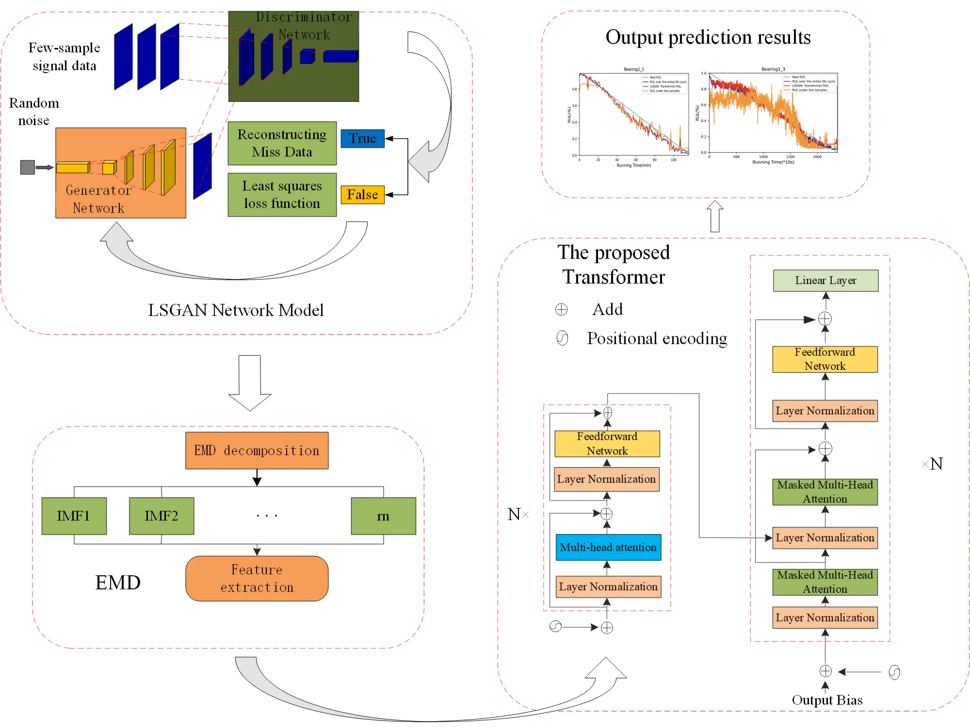
Highlights
- To address sample scarcity, we combine the Least Squares Generative Adversarial Network (LSGAN) with the Transformer model. A Dropout layer is added to the generator to prevent excessive parameters from affecting discrimination performance, further reducing overfitting in small sample training.
- To resolve excessive expected gradients after residual connections in the traditional Transformer, we move the layer normalization operation to the input of the decoder and encoder modules, creating a direct gradient path that effectively prevents the gradient vanishing problem.
- In the LSGAN model, we replace the cross-entropy loss function with the least squares loss function to avoid gradient vanishing and mode collapse during training, improving both the quality of generated samples and the stability of the training process.
1. Introduction
With the rapid progress of the modern machinery industry, the complexity and precision of bearings have increased significantly [1]. The safe operation of bearings in engineering applications is crucial, and real-time monitoring and analysis of their health status has become essential. Therefore, prognostic health management (PHM) technology has gradually received widespread attention from academia and industry [2]. In PHM technology, accurate prediction of the remaining useful life (RUL) of bearings is an important part.
Remaining life prediction methods can generally be classified into three types: a failure mechanism model method, a data-driven method and a hybrid method that combines the two [3]. Given the complex structure and harsh working conditions of mechanical systems, establishing accurate failure mechanism models for life prediction is a huge challenge. The hybrid method is a prediction model that combines the advantages of two models. Currently, this method seems to be an excellent solution. However, it is very difficult to find a mechanism to integrate these two models. One of the main challenges of this approach is the need for dynamic data to continuously adjust the model [4]. The data-driven approach uses machine learning technology to mine the relationship between data features and remaining useful life (RUL). Unlike other methods that require complex physical models or expert systems, this approach mainly relies on the analysis of large amounts of sensor data for life prediction. This makes the data-driven approach gradually become the main trend in the field of RUL prediction [5]. Thanks to the continuous improvement of deep learning, such as convolutional neural networks [6], deep belief networks [7], and long short-term memory (LSTM) networks [8], they have been increasingly used in RUL prediction. For instance, Wang et al. [9] introduced a deep convolutional network (DSCN), and Li et al. [9] proposed using CNN to extract multi-scale features from the time and frequency domains of bearing vibration signals. Yang et al. [10] developed a dual CNN model for bearing remaining life prediction, in which the first CNN is used to identify the location of the initial fault, while the second CNN is responsible for predicting the remaining life. However, the main problem faced by data-driven methods is their dependence on a substantial amount of sensor data. In actual operation, the complex working environment of the equipment makes it difficult to collect certain status data on a large scale, resulting in the number of normal state data samples far exceeding the number of fault samples, which seriously affects the balance of the data. This poses a significant challenge to data-driven machine learning methods in bearing life prediction. In order to address the problem of insufficient and unbalanced data samples in bearing fault diagnosis and life prediction, generative adversarial networks (GANs) [11] have gained widespread attention in recent years because of their capacity to generate similar data based on real data.
The application of generative adversarial networks (GANs) can significantly address the challenge of insufficient one-dimensional time series or two-dimensional sample data during model training. By utilizing the competitive dynamics between the generating and discriminating networks, GANs can generate supplementary data, thereby alleviating issues of limited data volume or imbalance in bearing fault diagnosis and lifespan prediction. For example, David Verstraete et al. [12] used GAN networks, variational autoencoders (VAE) and adversarial-variational models to effectively predict bearing degradation and make comparisons. Xiang Li et al. [13] divided the entire life of the bearing into healthy stage and unhealthy stage, used the GAN network to generate data, and then provided the actual sample data and the generated data to CNN for feature extraction to predict the degradation process of the entire bearing life. He et al. [14] introduced an advanced deep autoencoder to tackle the issue of limited sample data, which demonstrated effective transfer learning performance. Gao et al. [15] use GAN basics to generate a very finite number of faults, generate a large number of faults, and then use a finite number of faults to generate a small number of faults. Hua et al. [16] proposed a GAN-based unbalanced data fault diagnosis method. It overcomes the fault diagnosis problem under sample imbalance. Zhou et al. [17] used a global optimization mechanism to update the GAN’s generator and adversary networks, enhancing the accuracy of fault diagnosis methods under conditions of limited and imbalanced data. Guo et al. [18] proposed a bearing imbalance dataset fault detection approach utilizing a Wasserstein distance conditional gradient penalty generative adversarial network. This method avoids the problems of gradient vanishing and slow model convergence during sample generation. The traditional GAN network method of expanding samples by generating data is prone to unstable training models and poor quality of generated samples. Due to the limitation of the cross entropy loss function in the network, gradient diffusion often occurs. In order to solve the problems of gradient dispersion, mode collapse and low data generation quality in the traditional GAN training process, He et al. proposed the Least Squares Generative Adversarial Networks (LSGAN) [19]. Based on GAN, this method improves the loss function of the discriminator from the original cross-entropy loss to the least squares loss, thereby alleviating the gradient vanishing problem and improving the quality of generated data. The core idea of LSGAN is to make the distribution of generated data closer to the real data distribution through the least squares loss function, and to improve the instability of GAN during training through a smooth gradient optimization process. Compared with traditional GAN, LSGAN avoids the gradient vanishing phenomenon caused by the cross entropy loss function in the original GAN through the least squares loss function, thereby making the training process more stable. In addition, the adversarial process between the generator and the discriminator of LSGAN is smoother, avoiding the common mode collapse problem in traditional GAN, which makes the generated data of higher quality, especially in terms of diversity and stability of data generation.
Although existing deep learning networks have been increasingly used in bearing remaining life prediction, and the introduction of GAN networks have effectively solved the problem of insufficient samples, they are not outstanding in capturing long-term dependencies or memories in condition monitoring data [20]. In order to solve this problem. Attention mechanisms, especially self-attention mechanisms [21], are increasingly widely used. The introduction of the Transformer network has led to its widespread use in natural language processing [22] and computer vision [23]. The Transformer is the latest sequence-to-sequence network model based on the self-attention mechanism. It uses parallel computing to obtain the dependency information between any vectors in a long time series, and has surpassed CNN and LSTM [24], [25] in time series analysis. Ru Chang et al. [26] invented a transformer combined with a multi-head probabilistic sparse self-attention mechanism to mine the degradation information inherent in the Hilbert marginal spectrum and predict the RUL of bearings. Su et al. [27] proposed a Transformer adaptive adjustment model to predict RUL. Ding et al. [28] proposed a convolutional transformer that combines convolution operations and self-attention mechanisms to estimate the RUL of the orientation.
In view of the main problems in the field of rolling bearing life prediction, first of all, the acquisition of rolling bearing vibration signal data under actual working conditions often faces many challenges: the complexity of the operating environment, the scarcity of fault data and the high cost of acquisition make the acquisition of a large amount of high-quality data a bottleneck restricting the accuracy of rolling bearing life prediction. Secondly, when processing long-time series vibration signals, traditional deep learning methods often have problems such as limited receptive field and insufficient ability to capture long-term dependencies, which makes it difficult for the model to fully explore the degradation law of rolling bearings and affects the accuracy of life prediction. We propose an LSGAN-Transformer model. The network adds a dropout layer to the generator G to avoid too many parameters affecting the network's discrimination results and avoid overfitting during small sample training. Using LSGAN to create sample data solves the problem that Transformer requires a large amount of signal data, while Transformer is responsible for concurrent processing of model data and focuses on specific data. When predicting long-life bearings, it helps to retain key features and improve the prediction accuracy of long-life bearings. In this paper, a series of layer normalization operations are added to the original Transformer network after the residual connection, which leads to the problem that the expected gradient of the output parameters near the model is too large when the model is initialized. It is proposed to move the normalization of the Transformer model layer to the input and residual networks in the decoder and encoder submodules, thereby forming a direct gradient path from input to output, avoiding the problem of excessive expected gradient of parameters near the output layer of the traditional Transformer network. The LSGAN-Transformer model proposed in this paper achieves relatively accurate RUL prediction for long-term series rolling bearing life prediction in the case a few samples.
2. Related theoretical models
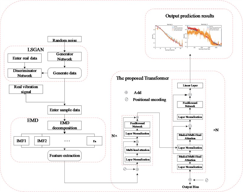
The model we proposed combines LSGAN and Trans-former, where LSGAN is used to generate samples similar to real data to solve the problem of inaccurate predictions caused by insufficient data in the case of small samples. Transformer is used to process long time series data to improve the accuracy of rolling bearing life prediction. Performing EMD decomposition on samples generated by LSGAN and real samples, extracting feature information from the signal, and inputting these features into the Transformer model for life prediction can further improve the efficiency and accuracy of the prediction. The process is shown in Fig. 1.
Fig. 1The proposed model process
2.1. LSGAN network theory
Lan Goodfellow et al. proposed the Generative Adversarial Network (GAN) in 2014 [29]. GAN is a deep learning model that has been increasingly used in recent years and has achieved remarkable application results in fields such as speech recognition [30], image restoration [31], data generation [32] and other fields. The generator is used to capture the underlying feature distribution of real data samples, and uses random noise signals as input to generate samples that are realistic enough to be easily mistaken for real samples. During the model training period, the two networks are constantly trained against each other. The optimization process of alternating training can be regarded as a minimax game problem. This method is used for learning, thereby continuously improving the performance of the adversarial generator and the discriminator. After a lot of training, the two will eventually reach a Nash equilibrium, and the objective function is:
where , are the generator network and the discriminator network respectively; is the objective function; is the real sample data input; is the random noise input of , and its distribution is ; is the generated sample data.
Traditional GAN networks use the cross entropy loss function to determine the difference between generated samples and real samples. However, the instability that occurs during model training often leads to phenomena such as gradient diffusion and mode collapse. In order to solve such problems that often occur in traditional GAN networks, Mao et al. [33] proposed the LSGAN model, which uses the least squares loss function to make the GAN network more stable and converge faster during training, and obtain higher quality generated data:
where: and are the labels of generated samples and real samples respectively; is the expected value of the discriminator for identifying the generated samples as true. and are the objective functions of the LSGAN discriminator and generator respectively; represents the real data distribution. In order to make the distribution of generated data and real data samples infinitely close, we set = 0, = = 1 and substitute them into the objective function of LSGAN to obtain:
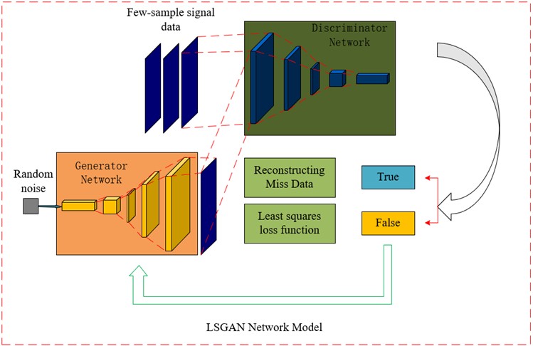
In the LSGAN network we proposed, a Dropout layer is added to the generator to prevent too many parameters from affecting the network discrimination effect. Dropout will randomly ignore the neurons in the generator, forcing other neurons in the network to participate in the generation process, avoiding overfitting during small sample training. In the discriminator, the least squares loss function is used, and through continuous iterative training, the generated samples gradually approach the spatial distribution of the real samples. The use of both will improve the quality of generated data, and this method can solve the problem of insufficient sample quantity. The proposed LSGAN model structure is shown in Fig. 2.
Fig. 2LSGAN network model
2.2. EMD decomposition
EMD (Empirical Mode Decomposition) is an adaptive data processing technique that is often used to process non-linear and non-stationary signals. Its main purpose is to de-compose complex signals into a series of simple oscillation modes, called intrinsic mode functions (IMFs) [34]. EMD does not rely on any preset basis functions, but decomposes according to the characteristics of the signal itself, and has strong adaptability. It automatically decomposes the signal into intrinsic mode functions (IMFs) representing different frequency components of the signal. Compared with traditional signal processing methods (such as Fourier trans-form), EMD can effectively process nonlinear and non-stationary signals. In recent years, for the processing of bearing vibration signals, EMD can finely distinguish different frequency components in vibration signals and has a high resolution for capturing and analyzing subtle fault features. Using EMD to decompose vibration signals and ex-tract features can be used for machine learning model training, fault diagnosis and prediction.
2.3. Transformer model theory
In the data-driven research on rolling bearing RUL prediction, sequence recurrent networks have been widely used, but these models perform poorly in serial operations and capturing long sequence dependencies, which restricts the further improvement of their operating efficiency and prediction accuracy. As a network model based on the self-attention mechanism, the Transformer model has a latecomer advantage in the above aspects. It is mainly divided into two parts: encoder and decoder. Both the encoder and decoder parts adopt a 6-layer stacked structure. Each layer of the encoder consists of a multi-head attention mechanism and a feedforward neural network. Each layer of the decoder consists of an occluded multi-head attention mechanism, an encoder-decoder multi-head attention mechanism, and a feedforward neural network.
The encoder is mainly used to encode the input rolling bearing feature sequence and add the temporal information of the sequence to the input vector through position encoding. The core part of its work is the multi-head attention mechanism, which is a variant of the attention mechanism. It mainly calculates the similarity between feature vectors by self-assigning weights to represent correlation, reducing dependence on external information, and thereby solving the problem of capturing long-distance dependencies. The transformer model proposed in this paper uses sine and cosine functions to implement position encoding. The details are as follows:
where: represents the position of the element in the vector; represents the dimension of the model; is the dimension.
For the encoder, it consists of two modules, a multi-head attention mechanism module and a fully connected feedforward neural network module. Residual connections are used in each module, and layer normalization is performed. The multi-head attention mechanism first processes the input time series data. This process can be regarded as a process of solving through a query vector and a set of key-value vector matrices. The query vector (), key vector () and weight vector () are converted from the previous output. The , , and matrices are calculated as:
where: , and are weight matrices. If , , and are used to represent the matrix dimensions, the above matrix can be expressed as:
where = . The subsequent attention calculation can be expressed as:
The attention calculation process is equivalent to solving the familiarity process of and , that is, calculating the cosine similarity and then normalizing it through the softmax function. The calculation of similarity is equivalent to calculating the weighted average of the input sequence, thereby identifying which parts of the input sequence are important. In the formula, plays a regulatory role in preventing the result after the softmax calculation from being either 0 or 1. Finally, the final attention is obtained by multiplying . It can be seen that attention is the recognition of input data and then obtaining important information through the mechanism of weight distribution. In order to pay attention to information from different positions together, further optimization is needed, using parallel attention calculations to learn different attention, improve the accuracy of the model, and finally splice all attention results. It can be expressed as:
where represents multi-head attention; represents its mapping matrix. The multi-head attention mechanism performs self-attention calculations without sharing parameters, so that the model can learn different information under different representations, and the role of residual connection is to prevent the gradient from being 0 when the model learning depth is too deep. The role of layer normalization is to map the vector value to the interval of 0~1, so as to speed up the convergence of the model. The specific calculation of layer normalization is:
where: is the output of layer normalization; and are the adjustment functions; and are the average value and standard deviation respectively.
For the decoder, the label data is first input into the occluded multi-head attention mechanism after position encoding, and then processed by addition and layer normalization as the query matrix . The output of the previous encoder is used as the key matrix and the value matrix to input the multi-head attention together, and finally processed by the feedforward neural network and output. Similar to the encoder, each sublayer of the decoder also uses residual connection and layer normalization. The difference is that when the decoder calculates the output, it cannot obtain the input time series of the subsequent time, so it needs to shield the input of the subsequent time. We call this method masking. Its calculation formula is:
where: represents masked multi-head attention and is the mask. Unlike the self-attention in the encoder, the self-attention in the decoder only focuses on the early positions in the output sequence. This is achieved by masking the future positions before computing the softmax step.
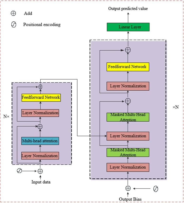
Since the original Transformer network model adds a series of layer normalization operations after the residual connection, the expected gradient of the parameters near the output layer is too large when the mode is initialized [35]. To address this issue, our proposed Transformer model moves layer normalization to the input of the decoder and encoder sub-modules and before the residual network. The resulting straight-through gradient path from input to output avoids the shortcomings of the traditional Transformer model in this regard. After this improvement, the output of the multi-head attention () and feedforward neural network () is:
In order to solve the problems of slow encoder convergence and unsatisfactory results in traditional network training, the Transformer model we proposed uses the GeLU activation function instead of ReLU activation function, which greatly improves the stability, generalization performance and training time of model training. Its structure diagram is shown in Fig. 3.
Fig. 3Transformer model proposed in this paper
3. Experimental verification
3.1. Dataset introduction
To assess the efficacy and progress of the proposed RUL prediction approach, we used the IEEE PHM Challenge 2012 rolling bearing dataset for experiments [36]. The dataset is collected by the PRONO-STIA experimental platform, and the collection device is shown in Fig. 4. A total of 17 bearing life cycle experiments were conducted. Among them, there were 7 bearings participating in the experiments under working conditions 1 and 2, and 3 bearings participating in the experiments under working conditions 3. Table 1 below introduces the PHM2012 dataset. According to relevant studies in the literature [37], [38], horizontal vibration signals usually provide more useful information than vertical vibration signals to track bearing degradation. Therefore, this paper only selects horizontal vibration signals for research.
Fig. 4PRONOSTIA acquisition platform
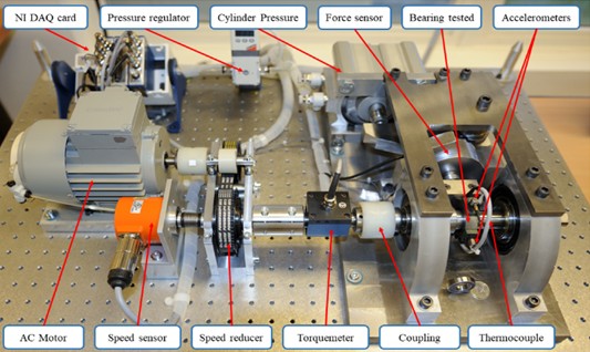
Table 1Introduction to the PHM2012 dataset
Operating conditions | Load / N | Rotating speed / (r/min) | Bearing No. |
Condition 1 | 4000 | 1800 | Bearing1-1~1-7 |
Condition 2 | 4200 | 1650 | Bearing 2-1~2-7 |
Condition 3 | 5000 | 1500 | Bearing 3-1~3-3 |
3.2. LSGAN network model training and sample generation
LSGAN can generate vibration signal data similar to actual working conditions. 15 % of the sample data of the tested bearing vibration signal is selected and input into LSGAN for training. After model iteration, generated samples are obtained and compared with the vibration signals of real samples. Fig. 5 is a comparison between some generated samples and real samples. It can be seen that the sample data generated by LGGAN has a highly consistent distribution pattern compared with the real sample data, indicating that the data generated by the model is of high quality and can effectively expand the bearing data set with missing data and improve the bearing life prediction performance of the model.
To better visualize the gap between the generated sample data and the real sample data, the Wasserstein distance is employed to compare the similarity between the two sets of bearing vibration signals. The Wasserstein distance serves as a metric for quantifying the difference between two probability distributions. The visual representation of the Wasser-stein distance for the two datasets is provided in Fig. 6. As illustrated in the figure, the probability distributions of the generated and real sample data are largely aligned, further validating the effectiveness of our proposed model.
Fig. 5Comparison between real data and generated data
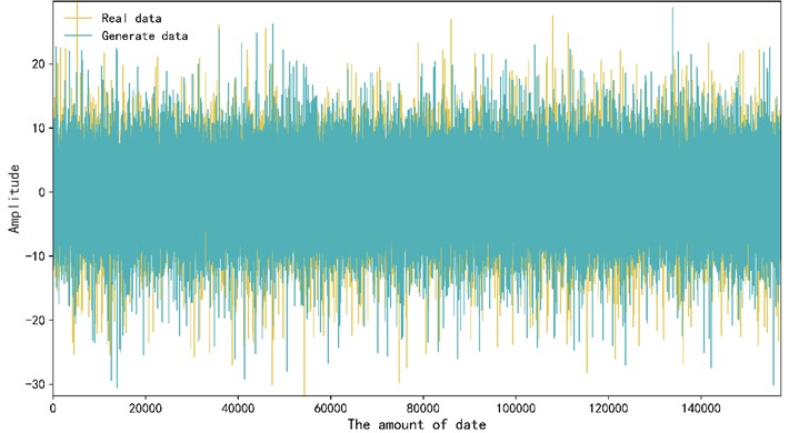
Fig. 6Probability distribution of generated data and real data
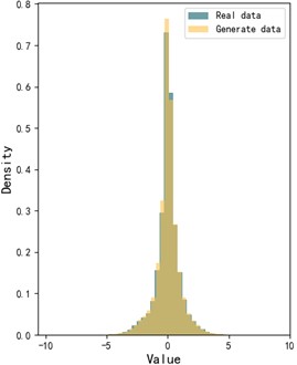
a) Histogram comparison
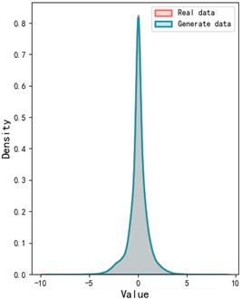
b) Kernel density estimation
3.3. EMD decomposition and transformer life prediction
This paper uses EMD (Empirical Mode Decomposition) to process real sample data and sample data generated by the LSGAN network, aiming to decompose complex bearing vibration signals into multiple intrinsic mode functions (IMFs) and residual signals of different frequency scales to extract more physically meaningful feature information. Since bearing vibration signals usually have non-stationary and nonlinear characteristics, direct feature extraction may be interfered by noise and complex signal components, thus affecting the accuracy of life prediction. EMD uses adaptive decomposition to enable high-frequency IMF components to capture the impact characteristics in the signal, medium-frequency IMFs to reflect periodic vibration information, and low-frequency IMFs and residual signals to reveal the overall operating trend, thereby retaining key state information at different scales while reducing noise interference. Based on the decomposed IMF and residual signals, 11 eigenvalues such as variance, mean, median, energy, RMS, Crest peak index, kurtosis index, straight line, entropy, arcsine feature, and arctangent feature are further extracted to fully characterize the time domain and frequency domain characteristics of the signal. Finally, the signal features after EMD decomposition are organized as time series and input into the proposed Transformer network for training and testing.
This paper follows the division of the PHM2012 data set and uses the bearings of working condition 1 in the data set. Each time, one of the seven bearing data under the working condition is selected as the test set of the model to test and predict its remaining life, and the remaining six bearing data are used as the training set of the model for training. To avoid the influence of accidental errors, each prediction task is repeated 5 times, and the average mean error and root mean square error are calculated as evaluation indicators. The experimental environment of this paper is python3.7, Pytorch1.8, and the computer configuration running this experimental environment is a 64-bit Windows system, i5-13400F, NVIDIA PTX2060. The model parameters are a training set epoch of 200, batch-size of 128, a learning rate of 0.0001, and test set batch-size of 128.
The specific operation is as follows: after the vibration signal data is generated by the LSGAN network, the generated samples are combined with the real samples for EMD decomposition, and the extracted IMF components, inverse hyperbolic sine function features, inverse tangent function features and other time domain data are used together with the corresponding time series as the input of the Transformer model for training.
This paper conducted a total of three groups of comparative verifications, which are the full life cycle prediction results of the prediction model proposed in this paper for bearings 1-1, 1-2, and 1-3 under working condition 1 and the bearing prediction results under the condition of few samples, as shown in Fig. 7.
Fig. 7Comparison of three cases from bearing 1-1 to bearing 1-3
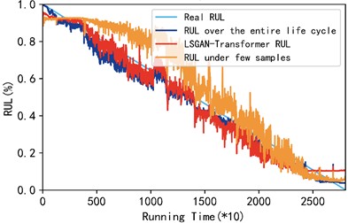
a) Comparison of the three cases of bearing 1-1
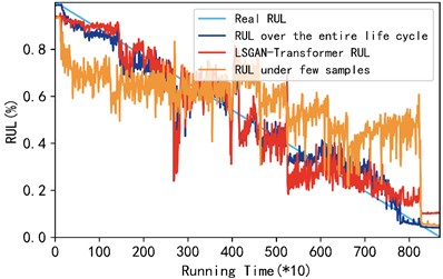
b) Comparison of the three conditions of bearing 1-2
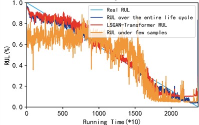
c) Comparison of the three cases of bearings 1-3
As shown in Fig. 7, the RUL of rolling bearings predicted by the LGGAN-Transformer model proposed in this paper is basically consistent with the prediction results under the full life cycle, while the prediction results under small samples show a large deviation, which proves the superiority of the model proposed in this paper in predicting the RUL of rolling bearings under small samples. In order to facilitate the observation of the accuracy comparison results of the three methods, this paper uses the mean absolute error (MAE) and mean root mean square error (RMSE) of the three test bearings as evaluation indicators. The data in Table 2 gives the gap between the three models in MES and RMSE. It can be seen intuitively from Table 2 that under the condition of small samples, after the support of the network proposed by us, its MSE and RMSE are improved by 58.63 % and 56.02 % respectively, which is slightly different from the prediction results under the full life cycle. It can be concluded that the model proposed in this paper has certain advantages in the prediction of rolling bearing life under small samples.
Table 2Comparison of MSE and RMSE results under three models
Model | MAE | RMSE |
Full life cycle | 0.0407 | 0.0534 |
LGGAN-Transformer | 0.0501 | 0.0636 |
Few samples | 0.1211 | 0.1446 |
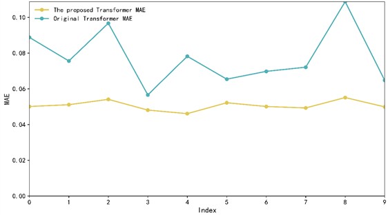
To highlight how the improved model in this paper outperforms the original Transformer model, we plotted the loss function diagrams for both models during their training processes and conducted ten paired experiments to observe the MAE change curves. Fig. 8 illustrates these changes.
As shown in Fig. 8, the loss curve of the improved Transformer model is smoother during training. Specifically, the loss curve comparison chart shows that the loss values of the improved model on the training set and test set are more stable, and the fluctuation is significantly reduced, indicating better convergence and stability. In addition, the MAE comparison chart shows that the improved model has less volatility and lower overall MAE during 10 training sessions, further proving its improved prediction accuracy. These results show that the improvements not only improve the prediction performance of the model, but also enhance the stability and generalization ability of the model.
Fig. 8Loss function and MAE change trend of bearing 1-1
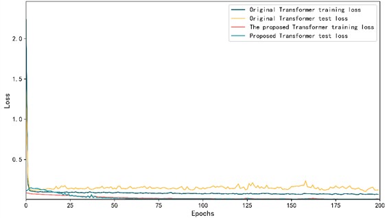
a) Loss curve comparison
b) MAE change trend
3.4. XJTU-SY dataset verification
To further confirm the general applicability of the proposed method, this study also validates it using the XJTU-SY dataset [39]. The test setup for this dataset is depicted in Fig. 9, which includes an AC motor, a motor speed controller, a rotating shaft, a support bearing, and a test bearing.
Fig. 9XJTU-SY rolling bearing test bench
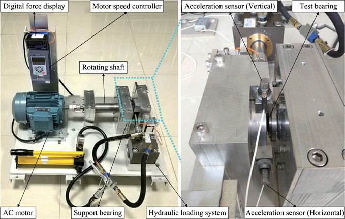
It can perform accelerated degradation experiments on bearings under different working conditions and obtain complete run-to-failure data. The experiment is designed with three working conditions, each with five bearings. This paper selects the bearings under working condition 1 for testing, and the test process is the same as the test process of the aforementioned PHM2012 dataset.
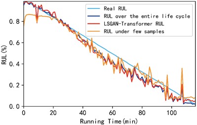
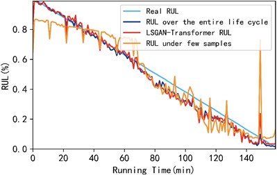
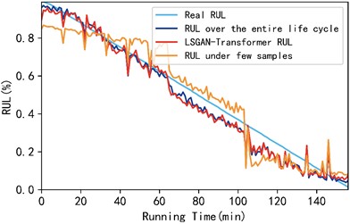
In each test, four bearings under Project 1 were selected as training sets and one bearing was selected as a test set. The LSGAN-Transformer model proposed in this paper was used for prediction. The prediction results under a few samples and full life cycle are compared in Fig. 10. Fig. 10 shows the RUL prediction results of bearings 1-1, 1-2, and 1-3 under working condition 1. In order to more intuitively show the accuracy comparison results of the three methods, this paper uses the mean absolute error (MAE) and mean root mean square error (RMSE) of the three test bearings as evaluation indicators to intuitively show the three prediction methods. The specific results are shown in Table 3.
Table 3Comparison of MSE and RMSE results under three models
Model | MAE | RMSE |
Full life cycle | 0.0393 | 0.0420 |
LGGAN-Transformer | 0.0424 | 0.0519 |
Few samples | 0.0611 | 0.0810 |
As shown in Fig. 10 and Table 3, the mean absolute error (MAE) of the proposed method is improved by 30.61 % compared with the case of few samples; its root mean square error (RMSE) is improved by 35.93 % compared with the case of few samples. In addition, the mean absolute error and root mean square error of the rolling bearing RUL predicted by the proposed method on the XJTU-SY dataset are improved compared with the rolling bearing RUL predicted on the PHM2012 dataset, which further illustrates the superiority and universality of the proposed model.
Fig. 10Comparison results of three methods for XJTU-SY bearings 1-1 to 1-3
a) Comparison diagram of bearing 1-1 in three cases
b) Comparison of the three conditions of bearing 1-2
c) Comparison graphs of three conditions for bearings 1-3
3.5. Comparative experiment
This paper proposes the LSGAN-Transformer model for rolling bearing life prediction under small samples and improves its structure. To clearly illustrate the advantages of the proposed model compared to conventional methods, existing commonly used prediction methods are selected for comparative experiments, namely LSTM model, BiLSTM model, CNN-Transformer model, Bi-TCN-LSTM model and the LSGAN-Transformer model proposed in this paper. The mean absolute error (MAE) and average root mean square error (RMSE) of several models are shown in Fig. 11.
Fig. 11Comparison of MAE and RMSE of five models
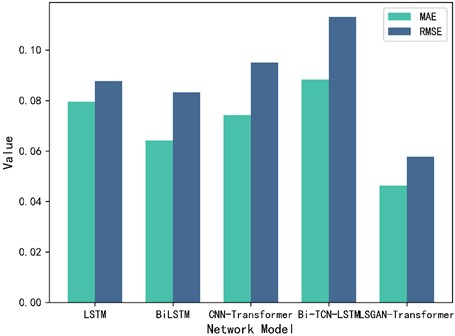
As shown in Fig. 11, the comparative experiments of the five models show that the prediction results of the method proposed in this paper have the best MAE and RMSE performance compared with the four commonly used models. Compared with the optimal BiLSTM network model, its MAE is improved by 27.78 % and RMSE is improved by 30.52 %. It is further verified that the model proposed in this paper not only has good prediction effect under small samples, but also has certain advantages compared with other commonly used models.
4. Conclusions
Aiming at the problem that vibration signals are difficult to collect under actual operating conditions of rolling bearings and the proportion of collected signal samples is unbalanced, a rolling bearing remaining life prediction method based on LSGAN-Transformer model is proposed. The following conclusions are obtained through experimental verification:
1) To address the problem of rolling bearing RUL being difficult to predict when there is little sample data and an unbalanced sample ratio, we introduced the LSGAN network model and added a dropout layer to its generator to prevent too many parameters from affecting the network's discrimination effect, thereby avoiding the overfitting phenomenon that often occurs during small sample training. The least squares loss function is used in the discriminator to replace the function in the traditional GAN, making the model more stable during training and accelerating the convergence of the model. Experimental results show that the quality of the generated samples is very close to that of the real samples.
2) In order to solve the problem that the expected gradient of the parameters near the output layer is too large when adding some column layer normalization after the residual connection during model initialization in the traditional Transformer model, this paper proposes to move the Transformer model layer normalization to the input of the decoder and encoder submodules and before the residual network, thereby forming a direct gradient path from input to output, which effectively avoids this problem. Considering that the encoder converges slowly and the effect is not ideal, we use the GeLU activation function instead of the traditional ReLU activation function, which improves the stability of the model during training.
3) Experimental verification of the proposed model shows that: compared with the prediction results under small sample conditions, the MAE and RMSE of this paper on the PHM2012 dataset are improved by 59.63 % and 56.02 % respectively, and the prediction results are basically consistent with the results of vibration signals under the full life cycle; compared with the prediction results of other common models, the MAE and RMSE are improved by 21.8 % and 23.56 % respectively, which further proves the effectiveness and superiority of our proposed model in the prediction of rolling bearing RUL.
4) To prove the universality of our proposed model, we conducted a comparative verification on the XJTY-SY dataset. The results show that the proposed model’s prediction results (MAE) and RMSE) on the XJTY-SY dataset are improved by 30.61 % and 35.93 % respectively compared with those under few samples; compared with the PHM2012 dataset, the MAE and RMSE on this dataset are also improved, further verifying the universality of this method.
References
-
L. W. Wang, X. C. Luan, and Y. D. Shua, “Fault extraction of roller bearing outer ring scratch in the complex path based on fast ICA,” (in Chinese), Machinery Design and Manufacture, Vol. 12, pp. 77–81, Dec. 2021.
-
Y. Lei, N. Li, S. Gontarz, J. Lin, S. Radkowski, and J. Dybala, “A model-based method for remaining useful life prediction of machinery,” IEEE Transactions on Reliability, Vol. 65, No. 3, pp. 1314–1326, Sep. 2016, https://doi.org/10.1109/tr.2016.2570568
-
W. Peng, Z.-S. Ye, and N. Chen, “Joint online RUL prediction for multivariate deteriorating systems,” IEEE Transactions on Industrial Informatics, Vol. 15, No. 5, pp. 2870–2878, May 2019, https://doi.org/10.1109/tii.2018.2869429
-
R. Zhao, R. Yan, Z. Chen, K. Mao, P. Wang, and R. X. Gao, “Deep learning and its applications to machine health monitoring,” Mechanical Systems and Signal Processing, Vol. 115, pp. 213–237, Jan. 2019, https://doi.org/10.1016/j.ymssp.2018.05.050
-
H. Liu, D. Yao, and J. Yang, “Fault diagnosis of rolling bearing based on multi branch depth separable convolutional neural network,” (in Chinese), Journal of Vibration and Shock, Vol. 40, No. 10, pp. 95–102, Oct. 2021.
-
X. Li, W. Zhang, and Q. Ding, “Deep learning-based remaining useful life estimation of bearings using multi-scale feature extraction,” Reliability Engineering and System Safety, Vol. 182, pp. 208–218, Feb. 2019, https://doi.org/10.1016/j.ress.2018.11.011
-
G. E. Hinton, S. Osindero, and Y.-W. Teh, “A fast learning algorithm for deep belief nets,” Neural Computation, Vol. 18, No. 7, pp. 1527–1554, Jul. 2006, https://doi.org/10.1162/neco.2006.18.7.1527
-
X. Chen and Z. Liu, “A long short-term memory neural network based Wiener process model for remaining useful life prediction,” Reliability Engineering and System Safety, Vol. 226, p. 108651, Oct. 2022, https://doi.org/10.1016/j.ress.2022.108651
-
B. Wang, Y. Lei, N. Li, and T. Yan, “Deep separable convolutional network for remaining useful life prediction of machinery,” Mechanical Systems and Signal Processing, Vol. 134, p. 106330, Dec. 2019, https://doi.org/10.1016/j.ymssp.2019.106330
-
J. Zhu, N. Chen, and W. Peng, “Estimation of bearing remaining useful life based on multiscale convolutional neural network,” IEEE Transactions on Industrial Electronics, Vol. 66, No. 4, pp. 3208–3216, Apr. 2019, https://doi.org/10.1109/tie.2018.2844856
-
G. Yang, L. Liu, and C. Xi, “Bearing fault diagnosis based on SA-ACGAN data generation model,” (in Chinese), China Mechanical Engineering, Vol. 33, No. 13, pp. 1613–1621, 2022.
-
D. Verstraete, E. Droguett, and M. Modarres, “A deep adversarial approach based on multi-sensor fusion for semi-supervised remaining useful life prognostics,” Sensors, Vol. 20, No. 1, p. 176, Dec. 2019, https://doi.org/10.3390/s20010176
-
X. Li, W. Zhang, H. Ma, Z. Luo, and X. Li, “Data alignments in machinery remaining useful life prediction using deep adversarial neural networks,” Knowledge-Based Systems, Vol. 197, p. 105843, Jun. 2020, https://doi.org/10.1016/j.knosys.2020.105843
-
H. Zhiyi, S. Haidong, J. Lin, C. Junsheng, and Y. Yu, “Transfer fault diagnosis of bearing installed in different machines using enhanced deep auto-encoder,” Measurement, Vol. 152, p. 107393, Feb. 2020, https://doi.org/10.1016/j.measurement.2019.107393
-
Y. Gao, X. Liu, and J. Xiang, “FEM simulation-based generative adversarial networks to detect bearing faults,” IEEE Transactions on Industrial Informatics, Vol. 16, No. 7, pp. 4961–4971, Jul. 2020, https://doi.org/10.1109/tii.2020.2968370
-
F. Hua, “Rolling bearing anomaly detection based on generative adversarial networks,” (in Chinese), Artificial Intelligence and Robotics Research, Vol. 8, No. 4, pp. 208–218, Jan. 2019, https://doi.org/10.12677/airr.2019.84023
-
F. Zhou, S. Yang, H. Fujita, D. Chen, and C. Wen, “Deep learning fault diagnosis method based on global optimization GAN for unbalanced data,” Knowledge-Based Systems, Vol. 187, p. 104837, Jan. 2020, https://doi.org/10.1016/j.knosys.2019.07.008
-
G. Junfeng, W. Miaosheng, and S. Lei, “New method of fault diagnosis for rolling bearing imbalance data set based on generative adversarial network,” (in Chinese), Computer Integrated Manufacturing System, Vol. 28, No. 9, p. 2825, 2022.
-
X. Mao, Q. Li, H. Xie, R. Y. K. Lau, Z. Wang, and S. P. Smolley, “Least squares generative adversarial networks,” in IEEE International Conference on Computer Vision (ICCV), pp. 2813–2821, Oct. 2017, https://doi.org/10.1109/iccv.2017.304
-
P. Shaw, J. Uszkoreit, and A. Vaswani, “Self-attention with relative position representations,” arXiv:1803.02155, Jan. 2018, https://doi.org/10.48550/arxiv.1803.02155
-
Y. Cao, Y. Ding, M. Jia, and R. Tian, “A novel temporal convolutional network with residual self-attention mechanism for remaining useful life prediction of rolling bearings,” Reliability Engineering and System Safety, Vol. 215, p. 107813, Nov. 2021, https://doi.org/10.1016/j.ress.2021.107813
-
J. Devlin, M.-W. Chang, K. Lee, and K. Toutanova, “Pre-training of deep bidirectional transformers for language understanding,” Proceedings of the 2019 Conference of the North, Vol. 3, No. 8, Jan. 2019, https://doi.org/10.18653/v1/n19-1423
-
K. Han, A. Xiao, and E. Wu, “Transformer in transformer,” Advances in Neural Information Processing systems, Vol. 34, pp. 15908–15919, 2021.
-
J. Luo and X. Zhang, “Convolutional neural network based on attention mechanism and Bi-LSTM for bearing remaining life prediction,” Applied Intelligence, Vol. 52, No. 1, pp. 1076–1091, May 2021, https://doi.org/10.1007/s10489-021-02503-2
-
T. Tian, C. Song, J. Ting, and H. Huang, “A French-To-English machine translation model using transformer network,” Procedia Computer Science, Vol. 199, pp. 1438–1443, Jan. 2022, https://doi.org/10.1016/j.procs.2022.01.182
-
Y. Chang, F. Li, J. Chen, Y. Liu, and Z. Li, “Efficient temporal flow transformer accompanied with multi-head probsparse self-attention mechanism for remaining useful life prognostics,” Reliability Engineering and System Safety, Vol. 226, p. 108701, Oct. 2022, https://doi.org/10.1016/j.ress.2022.108701
-
X. Su, H. Liu, L. Tao, C. Lu, and M. Suo, “An end-to-end framework for remaining useful life prediction of rolling bearing based on feature pre-extraction mechanism and deep adaptive transformer model,” Computers and Industrial Engineering, Vol. 161, p. 107531, Nov. 2021, https://doi.org/10.1016/j.cie.2021.107531
-
Y. Ding and M. Jia, “Convolutional transformer: an enhanced attention mechanism architecture for remaining useful life estimation of bearings,” IEEE Transactions on Instrumentation and Measurement, Vol. 71, pp. 1–10, Jan. 2022, https://doi.org/10.1109/tim.2022.3181933
-
I. J. Goodfellow et al., “Generative adversarial nets,” Advances in Neural Information Processing Systems, Vol. 27, 2014.
-
S. Pascual, A. Bonafonte, and J. Serrà, “SEGAN: speech enhancement generative adversarial network,” arXiv:1703.09452, Jan. 2017, https://doi.org/10.48550/arxiv.1703.09452
-
C. Ledig et al., “Photo-realistic single image super-resolution using a generative adversarial network,” in IEEE Conference on Computer Vision and Pattern Recognition (CVPR), pp. 105–114, Jul. 2017, https://doi.org/10.1109/cvpr.2017.19
-
A. Radford, L. Metz, and S. Chintala, “Unsupervised representation learning with deep convolutional generative adversarial networks,” arXiv:1511.06434, Jan. 2015, https://doi.org/10.48550/arxiv.1511.06434
-
R. Xiong, Y. Yang, and D. He, “On layer normalization in the transformer architecture,” in International conference on machine learning, pp. 10524–10533, 2020.
-
N. E. Huang et al., “The empirical mode decomposition and the Hilbert spectrum for nonlinear and non-stationary time series analysis,” Proceedings of the Royal Society of London. Series A: Mathematical, Physical and Engineering Sciences, Vol. 454, No. 1971, pp. 903–995, Mar. 1998, https://doi.org/10.1098/rspa.1998.0193
-
L. Liu, X. Liu, J. Gao, W. Chen, and J. Han, “Understanding the difficulty of training transformers,” arXiv:2004.08249, Jan. 2020, https://doi.org/10.48550/arxiv.2004.08249
-
P. Nectoux, R. Gouriveau, and K. Medjaher, “PRONOSTIA: An experimental platform for bearings accelerated degradation tests,” in IEEE International Conference on Prognostics and Health Management, PHM’12, pp. 1–8, 2012.
-
A. Soualhi, K. Medjaher, and N. Zerhouni, “Bearing health monitoring based on Hilbert-Huang transform, support vector machine, and regression,” IEEE Transactions on Instrumentation and Measurement, Vol. 64, No. 1, pp. 52–62, Jan. 2015, https://doi.org/10.1109/tim.2014.2330494
-
R. K. Singleton, E. G. Strangas, and S. Aviyente, “Extended Kalman filtering for remaining-useful-life estimation of bearings,” IEEE Transactions on Industrial Electronics, Vol. 62, No. 3, pp. 1781–1790, Mar. 2015, https://doi.org/10.1109/tie.2014.2336616
-
B. Wang, Y. Lei, N. Li, and N. Li, “A hybrid prognostics approach for estimating remaining useful life of rolling element bearings,” IEEE Transactions on Reliability, Vol. 69, No. 1, pp. 401–412, Mar. 2020, https://doi.org/10.1109/tr.2018.2882682
About this article
The authors have not disclosed any funding.
The datasets generated during and/or analyzed during the current study are available from the corresponding author on reasonable request.
Fannian Meng: data curation, formal analysis, funding acquisition, resources, supervision, validation, writing-review and editing. Kaiwen Deng: conceptualization, data curation, formal analysis, investigation, methodology, software, validation, visualization, writing – original draft. Liujie Wang: conceptualization, data curation, formal analysis, investigation, methodology, project administration, resources, software, supervision, validation, visualization, writing-original draft. Jianhua Cui: funding acquisition, project administration, resources, supervision. Yahong Qian: funding acquisition, project administration, resources, supervision. Wenliao Du: funding acquisition, project administration, resources, supervision. Xiaoyun Gong: funding acquisition, project administration, resources, supervision. Liangwen Wang: funding acquisition, project administration, resources, supervision.
The authors declare that they have no conflict of interest.
