Correlation degree analysis of sliding bearing oil monitor data based on grey theory

Yuan, Huiwu; Zheng, Yuanchun; Guo, Linli; Wang, Jiayi; Liu, Xin

doi:10.21595/vp.2025.24740

Vibroengineering Procedia

Browse Procedia

Published: 15 May 2025

Check for updates

Correlation degree analysis of sliding bearing oil monitor data based on grey theory

Huiwu Yuan¹

Yuanchun Zheng²

Linli Guo³

Jiayi Wang⁴

Xin Liu⁵

^{1, 2, 3, 4}Sanya Quality and Technical Testing Station, Hainan Sanya, China

⁵Department of Basic, Naval University of Engineering, Hubei Wuhan, China

Corresponding Author:

Xin Liu

Cite the article Download PDF

Downloads 138

CrossRef Citations 1

Abstract

Based on regular analysis of the spectrum, PQ value, precision moisture content and kinematic viscosity of a certain sliding bearing lubricating oil, this paper used grey theory to study the correlation degree within these four kinds of analysis indicators. It is hoped that it can achieve mutual verification and judgment of the state evaluation of sliding bearings. It can provides reliable basis for studying the internal operating rules of sliding bearings. It can also provide scientific basis for the management and maintenance of sliding bearings.

1. Introduction

Sliding bearing was a complex frictional system with uncertainty [1-2]. Generally speaking, there were many theoretical methods for solving uncertainty problems, such as grey theory [3], probability and statistics theory [4], fuzzy theory [5] and rough set theory [6]. They were applied in different fields. Grey theory had distinct advantages in solving problems with unclear connotations among them [7]. It could use simple methods to study complex systems and obtain reliable analysis conclusions. In recent years it has been widely used in the fields of ships, railways, aviation and aerospace. Overall, the main application methods of grey system theory currently include grey correlation analysis [8], grey forecasting prediction [9], grey decision-making [10] and grey control.

Correlation degree was called as a measure of the magnitude of the correlation between two systems or two factors [11]. It described the relative changes in factors during the development process of the system. It was considered that the correlation was high if the relative changes between the two were basically the same during the system development process. Correlation analysis was a part of grey system theory which used grey correlation to describe the strength, magnitude and order of relationship between sequences. The greater the correlation was, the stronger the correlation was between the change factor and the reference factor. This reflected the greater the degree of mutual influence among various factors in the system.

The sliding bearings were mainly used to support the weight of each shaft and coupling, as well as the radial load generated during the rotation of the rotation of the shaft system, to ensure the normal operation of the shaft system. A sliding bearing was mainly consisted by shell components, bearing components, oil filling components, and connecting components. The used lubricating oil was Great Wall TSE68# turbine oil.

This article used grey theory to calculate the behavioral characteristics of various groups of lubricating oil in sliding bearings. The correlation degree was calculated using the measurement data of wear element content, PQ value, precision moisture and 40 ℃ kinematic viscosity of lubricating oil as the mother sequence and the measurement data of other items as the sub sequence. The purpose was to deeply study the relationship between different monitoring parameters in sliding bearing lubricating oil and provide scientific basis for the management and maintenance of sliding bearings.

2. Materials and methods

2.1. Acquisition of experimental data

Tracking and monitoring were carried out by using a sliding bearing lubricating oil as the monitoring object. Samples were taken and analyzed every 300 hours of operation. Each oil sample was tested for spectrum, PQ value, precision moisture, and 40℃ kinematic viscosity. Six main wear elements such as Fe, Cr, Pb, Cu, Sn, and Ni were mainly analyzed in the spectral analysis (unit: μg/g). The used instrument was a M-type oil emission spectrometer produced by American Hyperspectral Company. The PQ value was obtained using a TTL-M ferromagnetic abrasive particle tester produced by Shenzhen Yateks Optical Electronic Technology Co., Ltd. The precision moisture content (unit: μg/g) was tested using DL32 precision moisture tester produced by Mettler Toledo Technology Co., Ltd. The kinematic viscosity (unit: mm²/s) was tested using S-FLOW850 automatic viscometer produced by Omnitek in the Netherlands. The results were shown in Table 1.

Table 1The data of oil monitoring

S/N	Fe	Cr	Pb	Cu	Sn	Ni	PQ	Moisture	Viscosity
1	8.9	0.1	3.8	2.3	28	0.3
2	3.6	0.2	2.6	1.7	16.2	0
3	0.7	0.1	1.6	2.5	26.9	0	29	1588	66
4	7.2	0.2	0	2.5	43.7	1.2	42	163	67
5	1.5	0.1	0.5	2.1	26.3	0	32	283	64
6	8.0	0	0	1.4	22.1	0.1	35.5	536	68
7	3.5	0	0.2	1	7	0	23.5	328	61
8	10.4	0	0	1.9	26	0.7	30	367	68
9	6.6	0	0.4	1.8	17.9	0.3	45	717	65
10	5.0	0	0	0	15.7	0	45	159	65
11	9.7	0	0.9	1.6	22.7	0.3	30.5	92	65
12	9.4	0.1	0.1	1.3	22.8	0.4	44.5	115	64
13	7.8	0.5	1.6	1.2	20.3	0.1	31	948	64
14	7.2	0.1	0.3	0.9	16.5	0	18	384	64
15	8.8	0.5	2.0	1.2	19.5	0	36.5	641	66
16	10.7	0.1	10.1	10.2	19.2	0	37	421	66
17	10.3	0	1.1	6	19	0.5	26.5	200	67

Fig. 1Variation of wear element content in different metals

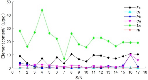
The changing trends of the six main wear elements, Fe, Cr, Pb, Cu, Sn, and Ni were showed in Fig. 1. It could be seen from Fig. 1 that the Fe element content was higher in the 8th, 16th and 17th tests. The Pb and Cu element content both were higher in the 16th test. The Sn element content was higher in the 4th test. The measured values of Cr and Ni element content were both smaller in each test.

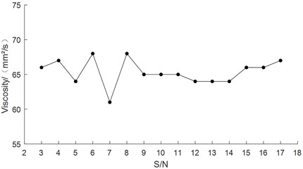
The change of trend chart of PQ value was showed in Fig. 2. The change of the trend chart of precision moisture content was showed in Fig. 3. The change of the trend chart of dynamic viscosity test was showed in Fig. 4. There were many results which could be seen from Figs. 2-4. The PQ value was relatively high at the 9th and 10th test which were both 45. The moisture content was the highest at the 3rd test which was 1588 μg/g. The results of the kinematic viscosity test at 40 ℃ did not change significantly with a minimum measurement of 61 mm²/s and a maximum measurement of 68 mm²/s.

Fig. 2The chart of PQ value trend

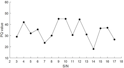
Fig. 3The chart of precision moisture content trend

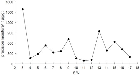
Fig. 4The chart of kinematic viscosity trend at 40 ℃

2.2. Calculation method for correlation degree

Correlation analysis generally includes following calculations and steps: (a) transformation of raw data, (b) calculation of correlation coefficients, (c) find the degree of closure, (d) arrange the closure sequence.

There are $m$ time series:

\begin{matrix} t & X_{1}^{(t)} & X_{2}^{(t)} & \dots & X_{n}^{(t)} \\ 1 & X_{1}^{(1)} & X_{2}^{(1)} & \dots & X_{n}^{(1)} \\ 2 & X_{1}^{(2)} & X_{2}^{(2)} & \dots & X_{n}^{(2)} \\ ⋮ & ⋮ & ⋮ & ⋮ & ⋮ \\ n & X_{1}^{(m)} & X_{2}^{(m)} & \dots & X_{n}^{(m)} \end{matrix}

That is $\{X_{1} (0) (t)\}$ , $\{X_{2} (0) (t)\}$ ,..., $\{X_{m} (0) (t)\}$ ( $t =$ 1, 2,..., $N$ ). $N$ is the length of each sequence, which is the number of data. These m sequences represent m factors (variables). Set another time series $\{X_{0} (0) (t)\}$ ( $t =$ 1, 2,..., $N$ ), which is called the mother sequence. The $m$ time series mentioned above are called sub sequences.

2.2.1. Data transformation: eliminate dimensions (or units) from the original data which were necessary and convert it into a comparable data sequence

A. Mean transformation: First, calculate the average of each sequence separately, and then remove the corresponding original data in each column from the average to obtain a new data column, which is the mean sequence. Each value is greater than 0, and most of them are close to 1. The sequence curves are interrelated intersection.

B. Initial value transformation: Use the first data of the same sequence to remove the subsequent raw data. A new multiple sequence is obtained, which is the initial value sequence. Each value is greater than 0 and the sequence has a common starting point.

C. Standardization transformation: First, calculate the mean and standard deviation of each sequence separately. Then subtract the mean from each original data and divide by the standard deviation. The new data sequence obtained in this way is the standardized sequence. The sequence mean is 0 and the variance is 1.

2.2.2. Calculate correlation coefficient

The mother sequence after data transformation is denoted as $\{X_{0} (t)\}$ . The child sequence is denoted as $\{X_{i} (t)\}$ . Therefore, the correlation coefficient $L_{0 i} (K)$ between the mother sequence $\{X_{0} (k)\}$ and the child sequence $\{X_{i} (k)\}$ can be calculated by Eq. (1) at time $t = k$ :

1

L_{0 i} (k) = \frac{∆_{m i n} + ∆_{m a x}}{∆_{0 i} (k) + ρ ∆_{m a x}},

where: $∆_{0 i} (k)$ represents the absolute difference between two comparison sequences at time $k$ , i.e. $∆_{0 i} (k) = |x_{0} (k) - x_{i} (k)|$ . $∆_{m a x}$ and $∆_{m i n}$ respectively represent the maximum and minimum absolute differences of all comparison sequences at each time step. Because of the comparison sequences intersect, $∆_{m i n} = 0$ is generally taken. $ρ$ is called the resolution coefficient, which means to weaken the distortion caused by the maximum absolute difference value being too large. It also can improve the significance of the difference between correlation coefficients. $ρ \in (0,1)$ and it is generally taken as 0.1-0.5.

The correlation coefficient reflects the degree of closeness between two compared sequences at a certain moment. For example at $∆_{m i n}$ moment, $L_{i 0} =$ 1, while at $∆_{m a x}$ moment, the correlation coefficient is at its minimum value. Therefore, the range of correlation coefficient is 0 $< L \leq$ 1.

2.2.3. Find correlation degree

From the above, it can be seen that correlation analysis is actually a geometric comparison of time series data. If two sequences coincide at each time point, that means the correlation number is equal to 1, then the correlation between the two sequences must also be equal to 1. On the other hand, the two comparison sequences cannot be perpendicular at any time, so the correlation coefficient is greater than 0 and the correlation degree is also greater than 0. Therefore, the correlation between the two sequences is calculated as the average of the correlation coefficients at each time point of the two comparison sequences. That is Eq. (2):

2

R_{0 i} = \frac{1}{N} \sum_{k = 1}^{N} L_{i 0} (k),

where $R_{i}$ represents the degree of association between subsoquence $i$ and mother sequence 0. $N$ represents the length of the comparison sequence (the number of data).

2.2.4. Sorting sequence

By arranging the correlation between m subsequences and the same mother sequence in order of magnitude, the maximum correlation factor can be determined with the parent sequence.

3. Results and analysis

3.1. Calculation of correlation degree of lubricating oil indicators for sliding bearings

The experimental data of sliding bearing lubricating oil were averaged firstly. The resolution coefficient is selected as $ρ = 0.5$ to calculate the correlation between indicators in various row in the Table 2. Fe element data were used as the mother sequence. Cr, Pb, Cu, Sn, Ni, PQ values, moisture and kinematic viscosity (40 ℃) were calculated and used as sub sequences. The correlation calculation results were shown in Table 2. The second row shows the correlation calculated using Cr as the mother sequence and Pb, Cu, Sn, Ni, PQ values, moisture, and 40C kinematic viscosity as sub sequences, and so on.

Table 2The correlation degree of lubricating oil indicators for sliding bearings

Correlation degree	Cr	Pb	Cu	Sn	Ni	PQ	Moisture	Viscosity
Fe	0.6977	0.6824	0.7377	0.8640	0.7168	0.7831	0.6492	0.4723
Cr		0.8722	0.7856	0.7200	0.8102	0.6020	0.8781	0.3837
Pb			0.8383	0.7036	0.7797	0.5958	0.8815	0.3941
Cu				0.7460	0.7803	0.6393	0.7723	0.4331
Sn					0.7417	0.7575	0.6726	0.4563
Ni						0.6295	0.8199	0.4213
PQ							0.6179	0.5581
Moisture								0.3958

3.2. Analysis

The data in column 8 of Table 2 are all greater than those in column 9 of the corresponding row. It was indicated that the concentration of elements such as Fe, Cr, Pb, Cu, Sn, Ni was more closely related to moisture than to kinematic viscosity in the lubricating oil of sliding bearings. This indicated that the moisture content in the lubricating oil of sliding bearings was closely related to wear. Controlling the moisture content was an important measure to prevent wear of sliding bearings.

The correlation between Fe and Sn, PQ values was high. The correlation between Sn and PQ values was high too in the tested sliding bearing lubricating oil. These indicated that they increased simultaneously during bearing wear. Fe was the substrate element of the rotating shaft. Sn was the substrate element of the bearing shell. PQ value was the quantity of ferromagnetic abrasive particles such as Fe and the friction. The rub between the shaft and the bearings could cause significant wear on the substrate which was consistent with objective reality.

The correlation between PQ value and kinematic viscosity was the highest among all wear indicators and kinematic viscosity. It was indicated that the amount of ferromagnetic abrasive particles had a significant impact on kinematic viscosity in the lubricating oil.

4. Conclusions

In the daily monitoring of sliding bearing lubricating oil, the following conclusions can be drawn: (1) Controlling the moisture content in the shaft lubricating oil was an important measure to prevent sliding bearing wear; (2) Special attention should be paid to the growth of wear indicators such as Fe, Sn, and PQ values. If there were abnormalities, timely measures should be taken to prevent excessive wear of sliding bearings; (3) We need to strengthen the monitoring of PQ values, and take timely measures to control any abnormalities to prevent accelerated deterioration of lubricating oil.

References

P. Qin, B. Yan, and R. Y. Song, “The condition monitoring of contacting fault of plain bearings,” China Mechanical Engineering, Vol. 13, No. 8, pp. 689–691, 2002.

Search CrossRef
A. R. Chen, “Fault Diagnosis technology for slide bearing based on Fourier Transform,” Bearing, No. 6, pp. 56–60, 2009.

Search CrossRef
Z. Y. Wang, Z. Li, and J. H. Wu, “On grey choice of the best measurement plan,” The Journal of Grey System, Vol. 9, No. 4, pp. 371–378, 1997.

Search CrossRef
S. Swaminathan and C. Smidts, “The event sequence diagram framework for dynamic probabilistic risk assessment,” Reliability Engineering and System Safety, Vol. 63, No. 1, pp. 73–90, 1999.

Publisher
S. Al-Sharhan, F. Karray, W. Gueaieb, and O. Basir, “Fuzzy entropy: a brief survey,” in 10th Annual IEEE Conference on Fuzzy Systems, Vol. 2, pp. 1135–1139, Oct. 2024, https://doi.org/10.1109/fuzz.2001.1008855

Publisher
Z. Pawlak, “Rough set theory and its application to data analysis,” Cybernetics and Systems, Vol. 29, No. 7, pp. 661–688, 1998.

Publisher
Z. Y. Wang, P. Qin, and Y. S. Gao, “Grey evaluation of measurement uncertainty,” The Journal of Grey System, Vol. 11, No. 4, pp. 347–352, 1999.

Search CrossRef
T. L. Tien, “A research on the deterministic grey dynamic model with multiple inputs DGDMMI (1, 1, 1),” Applied Mathematics and Computation, Vol. 139, pp. 401–416, 2003.

Publisher
D. Q. Truong and K. K. Ahn, “An accurate signal estimator using a novel smart adaptive grey model SAGM (1, 1),” Expert System with Applications, Vol. 39, No. 9, pp. 7611–7620, 2012.

Publisher
Y. Yang and D. Xue, “Continous fractional-order grey model and electricity prediction research based on the observation error feedback,” Energy, Vol. 115, pp. 722–733, 2016.

Publisher
C.-H. Lin, C.-H. Wu, and P.-Z. Huang, “Grey clustering analysis for incipient fault diagnosis in oil-immersed transformers,” Expert Systems with Applications, Vol. 36, No. 2, pp. 1371–1379, Mar. 2009, https://doi.org/10.1016/j.eswa.2007.11.019

Publisher

Cited by

A Method for Evaluating the Performance of Main Bearings of TBM Based on Entropy Weight–Grey Correlation Degree

(2025)

About this article

Received

21 December 2024

Accepted

24 January 2025

Published

15 May 2025

SUBJECTS

Materials and measurements in engineering

DOI

https://doi.org/10.21595/vp.2025.24740

Keywords

grey theory

correlation degree

sliding bearings

oil monitoring

Acknowledgements

The authors have not disclosed any funding.

Data Availability

The datasets generated during and/or analyzed during the current study are available from the corresponding author on reasonable request.

Conflict of interest

The authors declare that they have no conflict of interest.

This is an open access article distributed under the Creative Commons Attribution License, which permits unrestricted use, distribution, and reproduction in any medium, provided the original work is properly cited.

Previous article in issue Previous Next article in issue Next

Research article

2024 03 08

Mathematical simulation modeling analysis of sub-sea tunnel blasting based on grey correlation

Tingting Ling, Bolun Ding, Tingyao Wu

Research article

2024 02 17

Sector orifice with a correlation-based analysis

Santosh Kumar Panda

Research article

2022 09 21

Identification of initial fault time for bearing based on monitoring indicator, WEMD and Infogram

Jiadong Meng, Changfeng Yan, Tao Wen, Zonggang Wang

Research article

2020 11 21

Performance evaluation method of spherical bearing based on correlation and sensitivity analysis and SVM

Chen Liu, Yongjun Ni, Erli Gao, Wenxue Song

H. Yuan, Y. Zheng, L. Guo, J. Wang, and X. Liu, “Correlation degree analysis of sliding bearing oil monitor data based on grey theory,” Vibroengineering Procedia, Vol. 58, pp. 192–197, May 2025, https://doi.org/10.21595/vp.2025.24740

Copy Extrica

Copied to clipboard!

TY  - JOUR
DO  - 10.21595/vp.2025.24740
UR  - https://doi.org/10.21595/vp.2025.24740
TI  - Correlation degree analysis of sliding bearing oil monitor data based on grey theory
T2  - Vibroengineering Procedia
AU  - Yuan, Huiwu
AU  - Zheng, Yuanchun
AU  - Guo, Linli
AU  - Wang, Jiayi
AU  - Liu, Xin
PY  - 2025
DA  - 2025/05/15
PB  - Extrica
SP  - 192-197
VL  - 58
SN  - 2345-0533
SN  - 2538-8479
ER  - 

Copy Ris

Copied to clipboard!

 @article{Yuan_2025, title={Correlation degree analysis of sliding bearing oil monitor data based on grey theory}, volume={58}, ISSN={2538-8479}, url={https://doi.org/10.21595/vp.2025.24740}, DOI={10.21595/vp.2025.24740}, journal={Vibroengineering Procedia}, publisher={JVE International Ltd.}, author={Yuan, Huiwu and Zheng, Yuanchun and Guo, Linli and Wang, Jiayi and Liu, Xin}, year={2025}, month=may, pages={192–197} }

Copy Bibtex

Copied to clipboard!

[1]H. Yuan, Y. Zheng, L. Guo, J. Wang, and X. Liu, “Correlation degree analysis of sliding bearing oil monitor data based on grey theory,” Vibroengineering Procedia, vol. 58, pp. 192–197, May 2025, doi: 10.21595/vp.2025.24740.

Copy IEEE

Copied to clipboard!

Yuan, Huiwu, Yuanchun Zheng, Linli Guo, Jiayi Wang, and Xin Liu. “Correlation Degree Analysis of Sliding Bearing Oil Monitor Data Based on Grey Theory.” Vibroengineering Procedia 58 (May 15, 2025): 192–97. https://doi.org/10.21595/vp.2025.24740.

Copy Chicago

Copied to clipboard!

Correlation degree analysis of sliding bearing oil monitor data based on grey theory

Abstract

1. Introduction

2. Materials and methods

2.1. Acquisition of experimental data

2.2. Calculation method for correlation degree

2.2.1. Data transformation: eliminate dimensions (or units) from the original data which were necessary and convert it into a comparable data sequence

2.2.2. Calculate correlation coefficient

2.2.3. Find correlation degree

2.2.4. Sorting sequence

3. Results and analysis

3.1. Calculation of correlation degree of lubricating oil indicators for sliding bearings

3.2. Analysis

4. Conclusions

References

Cited by

About this article

Related Articles