Channel-attention-based time-frequency dual-branch network for bearing fault diagnosis in warehouse logistics sorting machines

Chen, Changhua; Deng, Xiangyang; Wan, Xinqi

doi:10.21595/jve.2026.26815

Journal of Vibroengineering

Browse Journal

Submit article

Published: October 30, 2026

Check for updates

Channel-attention-based time-frequency dual-branch network for bearing fault diagnosis in warehouse logistics sorting machines

Changhua Chen¹

Xiangyang Deng²

Xinqi Wan³

^{1, 2, 3}Xihua University, Chengdu, 610039, China

Corresponding Author:

Changhua Chen

Cite the article Download PDF

Article in Press

Downloads 24

Abstract

To address the difficulty of fully characterizing both local impacts and time-frequency information in bearing vibration signals from automated logistics sorting equipment using a single representation, this study develops a channel-attention-based time-frequency dual-branch fault diagnosis model. Each vibration window is represented both as a normalized one-dimensional time-series input and a two-dimensional continuous wavelet transform (CWT) time-frequency map. A temporal convolutional network (TCN) branch extracts local waveform and temporal variation features, while a multi-scale convolutional neural network (CNN) branch captures time-frequency textures at different receptive fields. Channel attention is introduced separately into the two branches to reweight informative features, and the two representations are concatenated for classification of normal, inner-race, outer-race, and rolling-element conditions. Experiments are conducted using bearing vibration records collected at 1200 r/min, with non-overlapping time windows used to construct training, validation, and held-out evaluation subsets. The proposed model achieves the highest mean accuracy and Macro-F1 among the baselines considered, and component ablation further supports the combined use of the dual-branch architecture, channel attention, and multi-scale feature extraction. The method provides an experimentally supported reference for bearing condition monitoring in warehouse logistics equipment.

Channel-attention-based time-frequency dual-branch network for bearing fault diagnosis in warehouse logistics sorting machines

Highlights

A time-frequency dual-branch network jointly learns from vibration signals and CWT maps.
Dilated TCN layers capture temporal patterns, while multi-scale CNN filters extract time-frequency textures.
Branch-specific channel attention reweights features before 256-dimensional concatenation.
Ablation tests support the contributions of channel attention and multi-scale convolution. 90 / 300 characters
The model reaches 98.33% mean accuracy and 0.9832 Macro-F1 on held-out windows at 1200 r/min.

1. Introduction

The logistics industry provides a fundamental link among production, distribution, and consumption. With the continued growth of e-commerce and manufacturing, warehousing and logistics have become increasingly important for improving material-flow efficiency and maintaining supply-chain stability. Feng and Ye [1] noted that digital and intelligent logistics operations are becoming an important means of improving logistics efficiency and supply-chain coordination. Bo et al. [2] investigated automated stereoscopic warehousing and further showed that intelligent warehouse equipment can improve storage and retrieval efficiency. Against this background, equipment reliability has become an important prerequisite for continuous warehouse operations.

Rolling bearings are key supporting components in rotating machinery such as motors, conveyor mechanisms, and automated sorting equipment, and their condition directly affects transmission stability. Local damage to the inner race, outer race, or rolling elements generally produces impacts, modulation effects, and changes in the frequency content of vibration signals. Randall and Antoni [3] systematically reviewed the vibration mechanisms and diagnostic principles associated with localized bearing defects and emphasized that the observed response depends on defect location, structural transmission paths, and operating condition. For warehouse logistics sorting equipment, continuous operation and frequent start-stop cycles further increase the need for reliable bearing-state identification. The present study uses logistics sorting equipment as the engineering application context, while the proposed method itself addresses vibration-based rolling-bearing condition identification and is not intrinsically limited to one type of machine.

Traditional bearing diagnosis commonly relies on time-domain statistics, spectra, and envelope-related features. Although these approaches provide useful physical interpretation, a single analysis domain may not simultaneously preserve the time location of transient impacts and their local frequency variation in non-stationary vibration signals. Peng and Chu [4] reviewed wavelet-transform applications in machine condition monitoring and fault diagnosis and showed the usefulness of wavelet analysis for local characterization of non-stationary signals. Yan et al. [5] further summarized wavelet-based methods for rotating-machinery fault diagnosis and highlighted their ability to represent localized time-frequency information. Building on this established foundation, CWT is used here to transform each one-dimensional vibration window into a two-dimensional time-frequency map, thereby providing a complementary representation of local spectral evolution alongside the original waveform.

With the development of deep learning, bearing fault diagnosis has gradually shifted from handcrafted feature design toward automatic representation learning. Zhang et al. [6] directly used raw vibration signals as the input to a deep model and demonstrated the feasibility of learning discriminative information from one-dimensional waveforms. Hoang and Kang [7] transformed vibration signals into image representations and used CNNs for classification, showing that two-dimensional vibration representations can support local texture extraction. Zhao et al. [8] reviewed deep learning for machine health monitoring, while Lei et al. [9] noted that data representation, feature-learning strategy, and operating-condition variation remain important factors affecting intelligent fault diagnosis. One-dimensional waveforms preserve sampling order and local impact evolution, whereas two-dimensional time-frequency maps emphasize how frequency components are distributed over time. To exploit this complementarity, recent studies have increasingly adopted multi-domain and multi-branch architectures. Xiong et al. [10] developed a multi-branch selective-fusion deep residual network to preserve complementary information while reducing redundancy among different information sources. Yasenjiang et al. [11] jointly modeled time- and frequency-domain information by combining ResNet, convolutional attention, BiGRU, and self-attention for dual-domain feature fusion. Liu et al. [12] further introduced channel attention into a dual-branch parallel network so that features extracted by different branches could be adaptively reweighted. These studies reflect a broader transition from single-path feature learning toward coordinated multi-representation modeling.

Attention mechanisms also provide an effective means of selectively emphasizing fault-related features. Hu et al. [13] proposed the squeeze-and-excitation (SE) network to model inter-channel dependencies and adaptively recalibrate channel responses. Woo et al. [14] subsequently proposed CBAM, which combines channel and spatial attention to emphasize informative responses. For bearing diagnosis, Wei and Yuan [15] integrated attention with a bidirectional recurrent structure to strengthen fault-related features in wind-turbine bearing vibration signals. Rezazadeh et al. [16] approached the problem from a domain-adaptation perspective and proposed a prototype-attention framework that weights target samples according to class prototypes, sample similarity, and prediction confidence while incorporating feature visualization to improve interpretability. As attention mechanisms evolve from simple channel reweighting toward multi-domain fusion and domain adaptation, the design of attention strategies that match different vibration representations remains an important issue.

Nevertheless, two issues remain in existing multi-domain and attention-based models. First, some methods combine residual networks, recurrent structures, self-attention, and multiple input domains simultaneously, making it difficult to determine which component is primarily responsible for performance gains. Second, one-dimensional vibration sequences and two-dimensional time-frequency maps have substantially different data organizations; applying identical encoders and weighting strategies to both representations may therefore fail to exploit their respective strengths. Rather than continuing to stack increasingly complex modules, it is useful to examine how temporal and time-frequency information complement each other, how branch-specific features should be selectively emphasized, and how individual structural components contribute to classification performance.

To address these issues, this study constructs a channel-attention-based time-frequency dual-branch bearing fault diagnosis model. For each vibration window, one branch retains the normalized one-dimensional waveform and uses a TCN with dilated convolution and residual connections to extract local impacts and temporal variations. The other branch applies CWT to the corresponding window and uses a CNN with parallel 3×3, 5×5, and 7×7 convolutions to capture time-frequency textures at different receptive fields. Because the one-dimensional temporal features and two-dimensional time-frequency features differ in organization, the two branches do not use identical weighting mechanisms. The TCN branch generates channel weights from global statistics of the temporal features, whereas the CNN branch uses two channel-attention modules at different feature depths to progressively recalibrate multi-scale time-frequency responses. Each branch produces a 128-dimensional feature vector, and the two vectors are concatenated into a 256-dimensional joint representation for four-class recognition of normal, inner-race fault, outer-race fault, and rolling-element fault states.

To determine whether the observed performance improvements can be associated with specific structural components rather than network complexity alone, controlled comparisons are conducted under a unified data split and training protocol. Four bearing vibration records acquired at 1200 r/min are segmented using non-overlapping windows and divided chronologically into training, validation, and held-out evaluation subsets. The experimental design includes time-series-only and time-frequency-only branches, removal of temporal attention, removal of time-frequency attention, removal of all attention modules, replacement of multi-scale convolution with a single-scale convolution, and alternative fusion strategies. These comparisons are used to assess the contributions of dual representation, branch-specific channel weighting, multi-scale feature extraction, and feature fusion.

2. Data acquisition and signal preprocessing

2.1. Bearing conditions and data acquisition

The rolling bearing of an automated sorting machine at Logistics Center L is used as the study object. Based on the available operating records, on-site inspection results, and maintenance records, four bearing states are considered: normal condition, inner-race fault, outer-race fault, and rolling-element fault. The normal state exhibits relatively low and stable vibration; inner-race faults show intermittent impact responses; outer-race faults exhibit more pronounced local pulses; and rolling-element faults display comparatively irregular responses that are more difficult to distinguish from time-domain amplitude alone.

The tested bearing is an SKF 6001 deep-groove ball bearing, and the experiment is conducted under an unloaded condition. The acquisition system consists of a mounted IEPE piezoelectric accelerometer, a USB-5801 dynamic signal acquisition module, and a LabVIEW host-computer program, as shown in Fig. 1. Panels (a) and (b) were photographed by Xiangyang Deng at Kunshan Hanjilong Measurement and Control Technology Co., Ltd., Kunshan, Jiangsu, China, in June 2025. Fig. 1(a) presents the bearing test rig and measurement point. The drive motor rotates the shaft through a coupling, the shaft is supported by the bearing support assembly, and the accelerometer is mounted at the right-side bearing support to record vibration during operation. Fig. 1(b) shows the USB-5801 acquisition module, through which the sensor output is digitized and transmitted to the host computer. Fig. 1(c) shows the LabVIEW acquisition interface. The sampling frequency is set to 10,240 Hz, and each acquisition is configured for 102,400 samples, corresponding to approximately 10 s. The interface displays the vibration waveform in real time and stores the acquired signal for subsequent sample construction and time-frequency analysis.

Fig. 1Experimental setup and vibration data acquisition system. Photos by Xiangyang Deng at Kunshan Hanjilong Measurement and Control Technology Co., Ltd., Kunshan, Jiangsu, China, in June 2025

Experimental setup and vibration data acquisition system. Photos by Xiangyang Deng at Kunshan Hanjilong Measurement and Control Technology Co., Ltd., Kunshan, Jiangsu, China, in June 2025

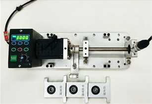
a) Experimental rig and measurement point

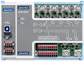
b) USB-5801 acquisition module

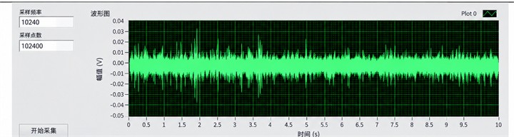
c) Raw acquisition interface: 10,240 Hz, 102,400 samples

The sampling frequency is set to 10,240 Hz, with a nominal acquisition duration of 10 s and 102,400 samples per record. Because the actually stored lengths differ slightly from the nominal settings, the present study uses the real number of stored samples to calculate record duration and construct model inputs. The record identifiers, actual sample counts, durations, and numbers of archived windows are summarized in Table 1.

Table 1Basic information on the four bearing vibration records

Category / Record ID	Nominal speed (r/min)	Stored samples	Duration (s)	Archived windows
Normal / Normal-R1	1200	102,312	9.9914	300
Inner-race fault / IF-R1	1200	101,808	9.9422	300
Outer-race fault / OF-R1	1200	102,312	9.9914	300
Rolling-element fault / BF-R1	1200	101,808	9.9422	300

As shown in Table 1, each bearing state corresponds to one source record with a duration of approximately 10 s. The original preprocessing workflow generated 300 archived windows per class, i.e., 1,200 windows in total; these windows are segments derived from the source records rather than independent acquisitions. The non-overlapping windows actually used in the revised analysis and their training, validation, and held-out evaluation allocation are described in Section 2.2.

2.2. Sliding-window segmentation and chronological sample partitioning

To convert the continuously acquired vibration records into fixed-length model inputs, a sliding-window strategy is used for signal segmentation. The revised sample construction directly uses the stored vibration sequences without applying an additional digital filter. The samples in the $j$ -th initial window are defined as follows:

1

w_{j} [n] = x [j S + n], n = 0, 1, \dots, L - 1, j = 0, 1, \dots, 299,

where $x [n]$ denotes the discrete vibration sequence; $w_{j} [n]$ is the $n$ -th sample in initial window $j$ ; $j$ is the initial-window index; $n$ is the sample index within the window; $L$ is the window length; $S$ is the sliding step; and $j S$ is the starting index of the window in the source record.

The original preprocessing used a window length of $L =$ 4,096 samples and a step size of $S =$ 326 samples, producing 300 initial windows for each class and 1,200 archived windows in total. The adjacent overlap ratio of these original windows is 92.0410 %.

To avoid assigning windows that share raw sample points to different data subsets, non-overlapping candidate windows are selected according to $j = 13 q$ , where $q = 0, 1, \dots, 23$ . The start-point spacing between adjacent candidates is therefore 13×326 = 4,238 samples, which is greater than the 4,096-sample window length and leaves 142 unused raw samples between adjacent candidate windows.

After selecting non-overlapping candidates, the training, validation, and held-out evaluation subsets are constructed according to chronological order within each source record. To introduce an additional temporal gap between adjacent subsets, candidate windows $q = 14$ and $q = 18$ are omitted. Consequently, 4,380 raw samples remain unused between the training and validation subsets and between the validation and held-out subsets. The same selection rule is applied to all four bearing states. The window indices, sample counts, and raw-sample ranges for each subset are listed in Table 2.

A total of 88 windows are ultimately used for model training and evaluation. Each class contains 14 training windows, 3 validation windows, and 5 held-out evaluation windows, with balanced class counts in all subsets. The training subset is used for parameter learning, the validation subset is used to monitor the training process, and the held-out subset is used only for final classification evaluation; it does not participate in parameter updating or checkpoint selection. This partition eliminates direct reuse of raw sample points across subsets. However, the windows of each class still originate from the same source record, so the reported results correspond to a within-record classification task under the current 1200 r/min condition.

Table 2Chronological partition of sliding-window samples

Subset	$q$ values ( $j = 13 q$ )	Per class	Total	Raw-sample range (inclusive)
Training	0-13	14	56	0-59, 189
Validation	15-17	3	12	63, 570-76, 141
Held-out evaluation	19-23	5	20	80, 522-101, 569
Total	–	22	88	–

Note: The same window-indexing rule is used for all four bearing records. $j$ denotes the initial-window index produced by the original preprocessing workflow, and $q$ denotes the non-overlapping candidate-window index. The window length is 4,096 samples and the original sliding step is 326 samples. Candidate windows $q = 14$ and $q = 18$ are reserved to create temporal gaps between adjacent subsets and are not included in training, validation, or held-out evaluation.

2.3. Data normalization

After sliding-window segmentation, each vibration window is independently normalized using min-max normalization to standardize the numerical range of the temporal-branch input. For non-constant windows, the samples are mapped to the interval [0, 1] as follows:

2

{\tilde{w}}_{j} [n] = \frac{w_{j} [n] - m i n (w_{j})}{m a x (w_{j}) - m i n (w_{j})}, n = 0, 1, \dots, L - 1,

where $w_{j} [n]$ denotes the original value at sample index $n$ in window $j$ , and ${\tilde{w}}_{j} [n]$ denotes the normalized value. $L$ is the window length defined in Section 2.2, and $m i n (w_{j})$ and $m a x (w_{j})$ are the minimum and maximum values of the current window. The extrema are calculated independently for each window rather than from the full dataset. After normalization, the minimum value of each non-constant window is mapped to 0 and the maximum value to 1.

This transformation standardizes the input range through amplitude translation and scaling while preserving the temporal order of the samples and the normalized waveform shape. However, because each window is scaled using its own extrema, absolute amplitude differences among windows are removed. Two windows that differ only by positive scaling and a constant offset can therefore become identical after normalization. Accordingly, the normalized temporal input is mainly used to learn waveform morphology and relative variation and should not be interpreted as a direct quantitative indicator of fault severity.

To examine whether this loss of absolute amplitude information affects classification, two control configurations are included: temporal z-score standardization using statistics derived from the training set, and an augmented input with standardized log-RMS and log-PTP amplitude descriptors. In both controls, the CWT image input is kept unchanged. The corresponding settings and results are reported in Section 4.3.3 and Table 8.

2.4. Continuous wavelet transform

To describe the local time-frequency distribution of the vibration signal, continuous wavelet transform (CWT) is applied to the same raw windows used by the temporal branch, producing the two-dimensional input for the CNN branch. The CWT is defined as:

3

W_{x} (a, b) = \frac{1}{\sqrt{|a|}} \int_{- \infty}^{\infty} x (t) ψ (\frac{t - b}{a}) d t,

where $x (t)$ is the vibration window to be transformed, $t$ is time, $W_{x} (a, b)$ is the wavelet coefficient, $a$ is the scale factor, $b$ is the translation parameter that determines the analysis position, and $ψ (\cdot)$ is the mother wavelet; the overbar denotes complex conjugation. A complex Morlet wavelet is used, with the following form:

4

ψ (u) = \frac{1}{\sqrt{π B}} e x p (- \frac{u^{2}}{B}) e x p (i 2 π C u),

where $u$ is the wavelet variable, $B$ is the bandwidth parameter, $C$ is the center-frequency parameter, and $i$ is the imaginary unit. The parameters are set to $B = 3$ and $C = 3$ , corresponding to the cmor3-3 configuration.

The discrete calculation uses $J = 256$ scales, and the scales and corresponding pseudo-frequencies are determined by:

5

a_{k} = \frac{2 F_{c} J}{k}, f_{k} = \frac{F_{c}}{a_{k} Δ t} = \frac{k f_{s}}{2 J}, k = 1, 2, \dots, J,

where $a_{k}$ is the k-th discrete scale and $f_{k}$ is its corresponding pseudo-frequency; $J = 256$ is the number of scales; $F_{c}$ is the center frequency of the mother wavelet used in the calculation; $f_{s}$ is the sampling frequency; and $Δ t = 1 / f_{s}$ is the sampling interval. With the settings used in the original preprocessing workflow, the frequency grid is 20, 40, ..., 5120 Hz, with a 20 Hz interval and an upper limit equal to the Nyquist frequency.

Each 4,096-sample window is converted by CWT into a 256×4,096 coefficient matrix. The coefficient magnitude is divided by the maximum coefficient magnitude of the corresponding window to obtain a normalized time-frequency amplitude map. The map is stored as an 875×656 RGB JPEG, resized to 64×64 pixels by bilinear interpolation, and scaled by dividing the pixel values by 255, yielding a 3×64×64 CNN input. The time-frequency image and the one-dimensional signal are paired by class and window index.

3. Channel-attention-based time-frequency dual-branch model

3.1. Overall architecture

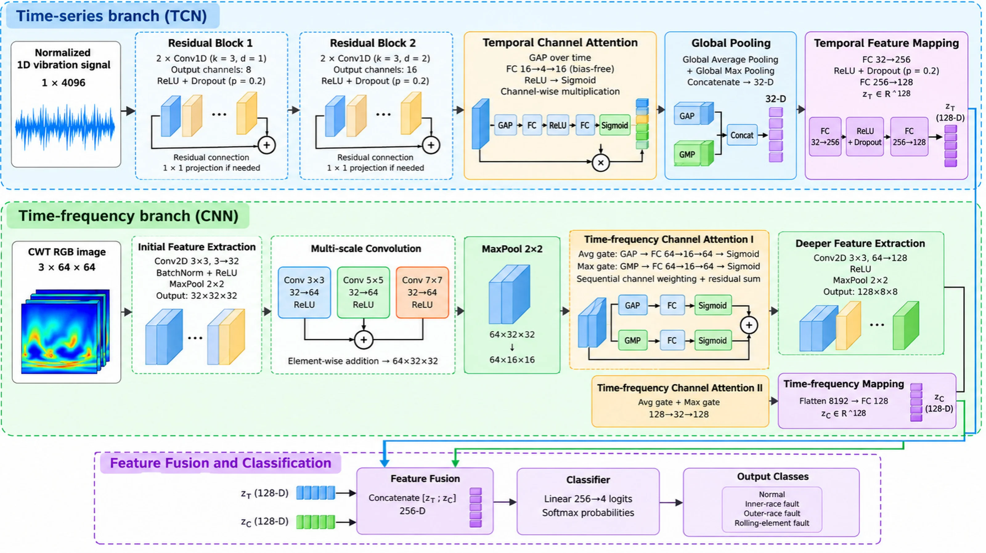
To jointly exploit temporal variations and local time-frequency distributions in bearing vibration signals, a channel-attention-based time-frequency dual-branch fault diagnosis model is constructed, as illustrated in Fig. 2. The model consists of a TCN temporal branch, a CNN time-frequency branch, channel-attention modules, a feature-fusion layer, and a classification layer. The paired inputs are the one-dimensional normalized signal and the two-dimensional CWT image corresponding to the same vibration window.

The TCN branch uses two sequential dilated-convolution residual blocks to extract local waveform and impact-related temporal features. The CNN branch uses parallel 3×3, 5×5, and 7×7 convolutions to capture multi-scale time-frequency textures, and the three responses are fused by element-wise addition. One channel-attention module is placed in the temporal branch, while two channel-attention modules are inserted at different depths in the time-frequency branch to adaptively recalibrate intermediate feature responses.

Fig. 2Overall architecture of the proposed channel-attention-based time-frequency dual-branch network for bearing fault diagnosis

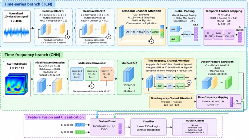
After pooling and feature mapping, the two branches each output a 128-dimensional feature vector. The two vectors are concatenated into a 256-dimensional joint representation, which is passed through a linear classification layer and Softmax to obtain the probabilities of the four bearing states: normal, inner-race fault, outer-race fault, and rolling-element fault. The operations, output dimensions, and trainable parameter counts of the major modules are summarized in Table 3.

3.2. TCN temporal feature branch

The TCN branch takes a normalized 1×4,096 vibration window as input and extracts local temporal features through two sequential residual blocks. Each block contains two dilated causal convolutions with a kernel width of 3. The dilation factors of the two blocks are 1 and 2, and the output-channel numbers are 8 and 16, respectively. The multi-channel dilated convolution can be expressed as:

6

v_{o, t} = β_{o} + \sum_{c = 1}^{C_{i n}} \sum_{r = 0}^{K - 1} h_{o, c, r} u_{c, t - d r},

where $u_{c, t}$ and $v_{o, t}$ denote the c-th input-channel feature and the o-th output-channel feature at time index t; $h_{o, c, r}$ is the convolution-kernel weight; $β_{o}$ is the bias; $C_{i n}$ is the number of input channels; $K$ is the kernel width; $r$ is the kernel-position index; and $d$ is the dilation factor. Inputs beyond the left sequence boundary are zero padded.

Table 3Layer-wise implementation and trainable parameter counts

Module	Main operations and settings	Output size	Parameters
Temporal branch: residual block 1	Two Conv1D layers, kernel 3, dilation 1; residual projection	8×4096	248
Temporal branch: residual block 2	Two Conv1D layers, kernel 3, dilation 2; residual projection	16×4096	1,328
Temporal branch: channel attention	Global average pooling; bias-free mapping 16→4→16; channel weighting	16×4096	128
Temporal branch: global pooling	Global average pooling + global max pooling; concatenation	32	0
Temporal branch: feature mapping	FC 32→256, ReLU, Dropout; FC 256→128	128	41,344
Time-frequency branch: initial extraction	3×3 conv, 3→32; BatchNorm, ReLU; 2×2 max pooling	32×32×32	960
Time-frequency branch: multi-scale convolution	Parallel 3×3, 5×5, 7×7 conv; 64 channels each; ReLU; element-wise addition	64×32×32	170,176
Time-frequency branch: pooling + attention I	2×2 max pooling; two independent mappings 64→16→64; channel weighting	64×16×16	4,256
Time-frequency branch: deeper extraction	3×3 conv, 64→128; ReLU; 2×2 max pooling	128×8×8	73,856
Time-frequency branch: attention II	Two independent mappings 128→32→128; channel weighting	128×8×8	16,704
Time-frequency branch: feature mapping	Flatten to 8192; FC 8192→128	128	1,048,704
Feature fusion and classification	Concatenate two 128-D features; FC 256→4	4	1,028
Total	Time-series/time-frequency dual-branch network	–	1,358,732

Zero padding followed by right-side cropping is used to preserve the sequence length. Each convolution is followed by ReLU and Dropout with a probability of 0.2. When required, a 1×1 convolution is used on the residual path to match the channel dimension, and the residual output is added to the main path and passed through ReLU.

The 16×4,096 feature map produced by the second residual block is first reweighted by temporal channel attention. Global average pooling and global max pooling are then applied separately, and the two pooled descriptors are concatenated into a 32-dimensional representation. This representation is mapped through fully connected layers 32→256→128 to obtain the temporal feature vector used for fusion with the CNN branch. ReLU and Dropout with a probability of 0.2 are applied between the two fully connected layers. The attention calculation is described in Section 3.4.1.

3.3. CNN time-frequency feature branch

The CNN branch takes the 3×64×64 CWT image constructed in Section 2.4 as input. A 3×3 convolution first maps the input to 32 channels, followed by batch normalization, ReLU, and 2×2 max pooling to produce a 32×32×32 feature map. Next, three parallel convolutions with kernel sizes 3×3, 5×5, and 7×7 each produce 64-channel outputs. After ReLU activation, the three responses are fused by element-wise addition:

7

U = \sum_{k \in {3, 5, 7}} R e L U ({C o n v}_{k \times k} (F)),

where $F$ is the feature map after the initial convolution and pooling, $k \times k$ denotes the convolution-kernel size, ${C o n v}_{k \times k} ()$ denotes a two-dimensional convolution with kernel size $k \times k$ , $R e L U ()$ is the activation function, and $U$ is the fused multi-scale feature. The three convolutions use a stride of 1 with paddings of 1, 2, and 3, respectively, so that their output sizes are identical. The summation therefore represents element-wise addition at corresponding spatial positions rather than channel concatenation. The fused output has the size 64×32×32.

The fused feature is reduced by 2×2 max pooling to 64×16×16 and then reweighted by time-frequency channel attention I. A subsequent 3×3 convolution, ReLU, and max pooling generate a 128×8×8 feature map, which is processed by time-frequency channel attention II. Finally, the feature map is flattened to 8,192 dimensions and mapped by a fully connected layer to a 128-dimensional time-frequency feature vector for fusion with the temporal representation.

3.4. Channel-attention mechanism

Channel attention is introduced separately into the TCN and CNN branches to adaptively reweight feature responses from the vibration waveform and the corresponding CWT image, thereby providing temporally and spectrally informative representations for subsequent fusion and classification.

3.4.1. Temporal channel-attention design

For the TCN branch, global average pooling is first applied to the temporal feature H produced by the second residual block. Two fully connected mappings are then used to generate channel weights, which are multiplied with the original feature map channel by channel:

8

g = σ (W_{2} ϕ (W_{1} G A P (H))), \tilde{H} = H ⊙ g,

where $H$ is the temporal feature extracted by the TCN from the vibration window, $\tilde{H}$ is the reweighted feature, $G A P (\cdot)$ denotes global average pooling along the temporal dimension, and $W_{1}$ and $W_{2}$ are bias-free fully connected weight matrices corresponding to a 16→4→16 mapping. ReLU and Sigmoid are denoted by $ϕ (\cdot)$ and $σ (\cdot)$ , respectively. The resulting 16-dimensional channel-weight vector is broadcast along the temporal dimension and multiplied with the feature map channel by channel.

3.4.2. Time-frequency channel-attention design

Two channel-attention modules are placed at the 64×16×16 and 128×8×8 feature-map stages of the CNN branch. For an input feature $F$ , an average-pooling gate first generates channel weight $a$ and produces an intermediate feature $X$ . Global max pooling is then applied to $X$ to generate the second channel weight $b$ , followed by second-stage weighting and residual combination:

9

a = σ (A_{2} (ϕ (A_{1} (G A P (F))))), X = F ⊙ a,

10

b = σ (B_{2} (ϕ (B_{1} (G M P (X))))), \tilde{F} = X ⊙ b + F ⊙ b,

where $G A P (\cdot)$ and $G M P (\cdot)$ denote global average pooling and global max pooling over the spatial dimensions, respectively; $a$ and $b$ are the two channel-weight vectors; $X$ is the first-stage weighted feature; and $\tilde{F}$ is the module output. $A_{1} / A_{2}$ and $B_{1} / B_{2}$ are two independent fully connected mappings with bias. The activation functions are the same as those used in Eq. (8), and the channel weights are broadcast over the spatial dimensions during multiplication. Both modules use $a$ reduction ratio of 4, with mappings 64→16→64 and 128→32→128, respectively, while preserving the input feature-map size.

3.5. Feature fusion and classification

After branch-specific feature extraction and channel reweighting, the 128-dimensional temporal feature $z_{T}$ and the 128-dimensional time-frequency feature $z_{C}$ corresponding to the same vibration window are concatenated into a joint representation. A linear classification layer and Softmax are then used for four-class bearing-state recognition:

11

z = [z_{T}; z_{C}] \in R^{256},

12

l = W z + b,

13

p_{c} = \frac{e x p (l_{c})}{\sum_{k = 1}^{4} e x p (l_{k})},

where $[\cdot; \cdot]$ denotes feature concatenation; $z$ is the resulting 256-dimensional fused feature; $W$ and $b$ are the weight matrix and bias of the classification layer; $l$ is the four-dimensional logit vector; $l_{c}$ is the logit for class $c$ ; and $p_{c}$ is the predicted probability that the current window belongs to class $c$ . The four classes are normal, inner-race fault, outer-race fault, and rolling-element fault, and the predicted label is the class with the highest probability.

3.6. Evaluation metrics

Accuracy, class-wise Precision, Recall, and F1-score are used to evaluate recognition performance, and Macro-F1 is used to summarize the four classes. Let the confusion matrix be $C$ , where $C_{i j}$ denotes the number of windows whose true class is $i$ and predicted class is $j$ :

14

A c c = \frac{\sum_{c = 1}^{4} C_{c c}}{\sum_{i = 1}^{4} \sum_{j = 1}^{4} C_{i j}},

15

P_{c} = \frac{C_{c c}}{\sum_{i = 1}^{4} C_{i c}},

16

R_{c} = \frac{C_{c c}}{\sum_{j = 1}^{4} C_{c j}},

where Accuracy denotes the overall classification accuracy; $P_{c}$ and $R_{c}$ are the Precision and Recall for class $c$ ; $C_{c c}$ is the number of correctly classified windows for class $c$ ; the corresponding column sum is the number of windows predicted as class $c$ ; and the row sum is the number of windows whose true class is $c$ . The class indices range from 1 to 4. Precision measures the correctness of predictions assigned to a class, whereas Recall measures the proportion of true samples of that class that are correctly identified.

The class-wise F1-score and Macro-F1 are calculated as:

17

F 1_{c} = \frac{2 P_{c} R_{c}}{P_{c} + R_{c}},

18

Macro-F1 = \frac{1}{4} \sum_{c = 1}^{4} F 1_{c},

where $F 1_{c}$ is the harmonic mean of Precision and Recall for class $c$ , and Macro-F1 is the unweighted mean of the four class-wise F1-scores. If a denominator is zero, the corresponding metric is defined as zero. The confusion matrix and class-wise metrics are also used to identify whether inner-race, outer-race, or rolling-element fault windows are misclassified as normal or as another fault class, avoiding reliance on overall accuracy alone.

Each neural-network configuration is trained independently using random seeds 42, 43, and 44, and the reported metrics are presented as the mean $\pm$ sample standard deviation. The same 20 held-out windows are used in all three runs, with five windows per class. The standard deviation therefore reflects optimization variability under a fixed data partition rather than variability across newly collected independent bearings. The same evaluation protocol is used for model comparison, class-wise analysis, and ablation experiments.

4. Experimental results and analysis

4.1. Experimental settings and comparison protocols

The experiments use the bearing vibration data collected at 1200 r/min as described in Section 2.1 and address four-class recognition of normal, inner-race fault, outer-race fault, and rolling-element fault states. Following the chronological partitioning scheme in Section 2.2, 56 training windows, 12 validation windows, and 20 held-out evaluation windows are constructed, with balanced class counts in each subset. All compared models use the same sample partition, so the reported results represent classification performance over different time segments of the existing records. The principal neural-network training settings are listed in Table 4.

Table 4Main neural-network training settings

Parameter	Setting
Optimizer	Adam
Initial learning rate	0.001
Loss function	Cross-entropy loss
Training epochs	50
Batch size	16
Learning-rate schedule	StepLR; multiplied by 0.5 every 20 epochs
Gradient clipping	Maximum L2 norm = 1.0
Regularization	Dropout = 0.2 in TCN convolutions and feature mapping; BatchNorm in the initial CNN block
Random seeds	42, 43, 44

To evaluate the proposed channel-attention-based time-frequency dual-branch model, experiments are conducted at two levels: model-structure comparison and component ablation. First, the complete dual-branch model is compared with a temporal-only branch, a time-frequency-only branch, a block-based GRU, a compact dual-domain adapted comparator, and a random forest (RF). The single-branch models retain the corresponding encoder and attention module and use a 128→4 classifier. The block-GRU model reshapes each 4,096-sample vibration window into 64 consecutive blocks and performs classification using a two-layer GRU followed by a fully connected layer. The RF uses 33 fixed time-domain and spectral descriptors and 200 decision trees. A compact dual-domain adapted model is also included as a structural reference; it contains separate temporal and frequency paths combined with a bidirectional GRU and self-attention. This comparator is an adapted reference implementation rather than an exact reproduction of any single published model.

Second, component ablations are performed using the complete dual-branch model as the reference. Temporal attention, time-frequency attention, and all attention modules are removed separately; the multi-scale convolution is replaced by a single 3×3 convolution; and feature concatenation is compared with mean fusion. Two amplitude-treatment controls are also included: temporal z-score standardization and additional log-RMS/log-PTP descriptors. Except for RF, all neural-network configurations use the training settings in Table 4 and are evaluated using the metrics defined in Section 3.6. The corresponding results are reported in Sections 4.3.1 and 4.3.3.

4.2. Bearing vibration signal characteristics

4.2.1. Time-domain characteristics

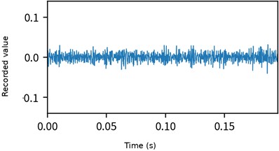
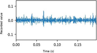
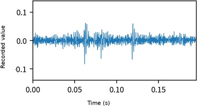
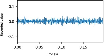
To compare the vibration responses of the four bearing states at 1200 r/min, the first 2,000 samples of the normal, inner-race fault, outer-race fault, and rolling-element fault records are plotted in the time domain, as shown in Fig. 3.

Fig. 3Time-domain waveforms of the four bearing states at 1200 r/min

a) Normal

b) Inner-race fault

c) Outer-race fault

d) Rolling-element fault

Fig. 3(a) shows that the normal record fluctuates mainly around zero within the displayed interval and does not exhibit impacts comparable in magnitude to those observed in the outer-race fault segment. In Fig. 3(b), the inner-race fault record contains local response increases superimposed on the background vibration; some peaks are more pronounced than those in the normal segment, although the short waveform alone is insufficient to establish a reliable impact repetition period. Fig. 3(c) shows more evident positive and negative amplitude excursions for the outer-race fault, with local impacts standing out clearly from the surrounding background. By contrast, the rolling-element fault segment in Fig. 3(d) does not show a sustained increase in amplitude, and its overall fluctuation range is relatively close to that of the normal segment. Thus, short-time amplitude alone does not provide a consistent basis for separating all four classes. These observations apply only to the displayed signal segments and should not be interpreted as universal behavior under all operating conditions.

To quantify amplitude-distribution differences across the complete stored records, the mean, sample standard deviation, root-mean-square value (RMS), peak-to-peak value, and excess kurtosis are calculated, as summarized in Table 5. The normal and outer-race fault records each contain 102,312 samples, while the inner-race and rolling-element fault records each contain 101,808 samples. Therefore, the extrema and statistics in Table 5 are not restricted to the first 2,000 samples shown in Fig. 3.

Table 5Statistics of the complete stored vibration records

Category	Mean	Sample standard deviation	RMS	Peak-to-peak	Excess kurtosis
Normal	0.000629	0.010992	0.011010	0.196033	1.3915
Inner-race fault	0.000634	0.011034	0.011052	0.158772	2.7258
Outer-race fault	0.000649	0.012660	0.012677	0.252243	8.0415
Rolling-element fault	0.000695	0.010307	0.010330	0.164785	1.3281

As shown in Table 5, the mean values of the four records range from 0.000629 to 0.000695, indicating only a small overall offset. The outer-race fault record has the largest sample standard deviation, RMS, peak-to-peak value, and excess kurtosis. Its RMS and peak-to-peak values are 0.012677 and 0.252243, respectively, approximately 15.14 % and 28.67 % higher than those of the normal record, and its excess kurtosis reaches 8.0415. Together with the local high-amplitude fluctuations in Fig. 3(c), this indicates stronger overall amplitude variation and more pronounced impulsive behavior in the current outer-race record. The inner-race fault has an RMS of 0.011052, close to the normal value of 0.011010, but its excess kurtosis is 2.7258 compared with 1.3915 for the normal record, while its peak-to-peak value of 0.158772 is lower than the normal value of 0.196033. Thus, its differences are not expressed as a simultaneous increase in all amplitude-related measures. The rolling-element fault has an RMS of 0.010330 and excess kurtosis of 1.3281, both slightly lower than the corresponding normal values, and therefore does not exhibit a simple amplitude-increase pattern. Overall, the outer-race record shows the most pronounced amplitude and impulsiveness in the present dataset, whereas the inner-race and rolling-element records remain close to the normal state in some statistical measures. These statistics describe the current records only and are not used as quantitative measures of physical defect severity.

Taken together, Fig. 3 and Table 5 show that local waveform behavior and full-record statistics describe different aspects of the current bearing signals. Because the normal, inner-race, and rolling-element records overlap in several amplitude-related measures, a single amplitude indicator is insufficient for reliable class identification. The following sections therefore examine the frequency content and its temporal evolution to motivate the joint use of the waveform and CWT representations, while classification performance is assessed using the held-out evaluation results.

4.2.2. Frequency-domain characteristics

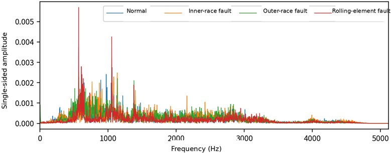
To compare the frequency composition of the four states, the first 4,096 samples of each record are selected. The mean of each window is removed before applying the fast Fourier transform (FFT), and the resulting single-sided amplitude spectra are shown in Fig. 4. With a sampling frequency of 10,240 Hz, the frequency resolution is 2.5 Hz and the analyzed range is 0-5120 Hz.

As shown in Fig. 4, the stronger spectral peaks of the four records are mainly concentrated in approximately the 500-1500 Hz range, while the amplitudes above 3500 Hz are generally low. Considerable spectral overlap exists among the classes, but local peak positions and amplitudes differ. In particular, the rolling-element fault window shows pronounced peaks near approximately 600 Hz and 1000 Hz. Although the RMS of the complete rolling-element fault record is lower than that of the normal record, a selected local window can still contain stronger spectral components; the two observations describe different quantities and are therefore not contradictory. The spectrum provides frequency-distribution information that is not directly visible from time-domain statistics alone.

These spectral differences describe only the selected windows and cannot be directly assigned to specific theoretical bearing characteristic frequencies without independently verified bearing geometry and corresponding measurements. In addition, a single FFT spectrum does not show how the response at each frequency evolves over time. CWT is therefore used in the next section to relate local waveform variation to its time-varying frequency distribution.

Fig. 4Single-sided FFT amplitude spectra of the four bearing vibration signals

4.2.3. Time-frequency characteristics

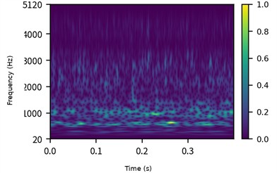
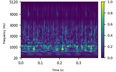
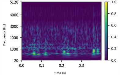
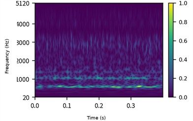
To examine how the major frequency components in Fig. 4 evolve over time, the same first 4,096 samples from each record are analyzed using the complex Morlet wavelet and zero-padded FFT-based linear convolution. The numerical support of the wavelet is set to [–8, 8]. With the 10,240 Hz sampling rate, the analysis window is 0.4 s long and spans 20-5120 Hz, as shown in Fig. 5.

Fig. 5Normalized CWT time-frequency amplitude maps of the four bearing states at 1200 r/min

a) Normal

b) Inner-race fault

c) Outer-race fault

d) Rolling-element fault

Fig. 5 was recomputed using the same analytical complex-Morlet formulation for qualitative visualization; model training uses the archived CWT images described in Section 2.4. Each subplot is normalized by its own maximum coefficient magnitude, so the colors indicate relative within-window response strength rather than absolute vibration energy across classes.

The stronger responses in Fig. 5 are mainly distributed in approximately the 500-1500 Hz range, consistent with the dominant spectral components in Fig. 4, while their temporal patterns and local textures differ. The normal segment exhibits low-frequency banded responses with localized amplitude variation. The inner-race fault segment shows multiple intermittent enhancement regions near approximately 1000 Hz. The outer-race fault segment exhibits more concentrated local high-response regions below 1000 Hz, with noticeable variation over time. The rolling-element fault segment presents a more continuous narrow-band response near approximately 600 Hz. These observations further indicate that similar frequency components can have different temporal distributions.

The time-domain, frequency-domain, and time-frequency analyses together show that the four bearing records differ not only in local waveform behavior but also in frequency composition and temporal spectral distribution. Accordingly, the proposed model uses the TCN branch to encode local temporal responses in the vibration window, the multi-scale CNN branch to encode CWT textures over different neighborhood sizes, and channel attention to recalibrate intermediate features. These signal observations provide the physical motivation for the dual-branch design, whose classification benefit is evaluated in Section 4.3 through single-branch comparisons and component ablations.

4.3. Model diagnosis analysis

4.3.1. Training process and overall performance

To examine the learning behavior of the complete dual-branch model, cross-entropy loss and classification accuracy are recorded over 50 training epochs. Fig. 6 shows the training and validation curves for random seed 42. The training and validation subsets contain 56 and 12 windows, respectively; the held-out evaluation subset is not used to generate the epoch-by-epoch curves. All neural-network configurations use the epoch-50 model for final evaluation.

Fig. 6Training and validation curves of the complete dual-branch model

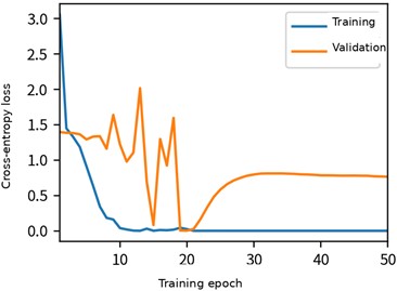
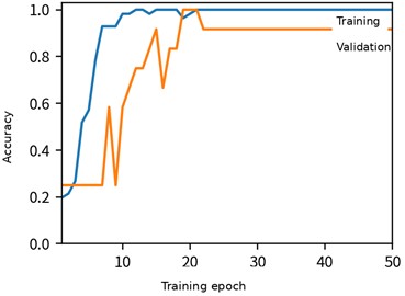
As shown in Fig. 6, the training loss decreases from 3.0562 to 0.0383 during the first 10 epochs, while the training accuracy reaches 98.21 %, indicating that the model rapidly fits the training data. After epoch 21, the training accuracy remains at 100 % and the loss approaches zero. In contrast, the validation process shows clearer fluctuations: the validation loss reaches 0.0020 at epoch 20 and subsequently increases to 0.7639 at epoch 50, while the validation accuracy reaches 100 % during epochs 19-21 and remains at 91.67 % from epoch 22 onward. The growing gap between training and validation performance indicates a tendency toward overfitting in the later training stage. Therefore, decreasing training error alone is not interpreted as continuing generalization improvement, and final model performance is assessed using the held-out evaluation results.

To evaluate overall classification performance, the complete dual-branch model is compared with the time-frequency-only branch, the time-series-only branch, the block-based GRU, the compact dual-domain adapted comparator, and RF according to the protocol defined in Section 4.1. All models are evaluated on the same 20 held-out windows. Mean accuracy and Macro-F1 over three random seeds are reported together with the number of trainable parameters and the average single-sample forward inference time, as shown in Table 6.

Table 6Classification performance and computational cost of different models

Configuration	Accuracy (%)	Macro-F1	Parameters	Forward time per sample (ms)
Complete dual-branch model	98.33±2.89	0.9832±0.0292	1,358,732	4.13
Time-frequency branch only (CNN)	90.00±0.00	0.8969±0.0054	1,315,172	3.57
Time-series branch only (TCN)	31.67±5.77	0.1816±0.0706	43,564	1.14
Block-based GRU	35.00±5.00	0.2746±0.0700	18,116	1.47
Compact dual-domain adapted comparator	66.67±2.89	0.6622±0.0323	29,684	3.61
RF (33 descriptors)	93.33±2.89	0.9328±0.0289	–	7.06

Table 6 shows that the proposed channel-attention-based time-frequency dual-branch model achieves a mean accuracy of 98.33 % and a Macro-F1 of 0.9832, the highest values among the listed models. Relative to the time-frequency-only CNN branch, the mean accuracy improves by 8.33 percentage points; relative to RF, the improvement is 5.00 percentage points. Because each single-branch comparator retains its corresponding encoder and attention module, the comparison mainly reflects the benefit of joint temporal and time-frequency encoding over either representation alone. The observed advantage is therefore based on the actual classification results of the complete model under the current training protocol rather than on the dual-branch label itself.

The results in Table 6 summarize overall performance on the current held-out windows but do not reveal which classes account for the remaining errors or isolate the contributions of attention and multi-scale convolution. Section 4.3.2 therefore reports class-wise metrics and a confusion matrix, while Section 4.3.3 uses controlled ablations and amplitude-treatment comparisons to examine the roles of the individual design choices.

4.3.2. Class-wise recognition and misclassification analysis

To characterize the recognition behavior of the complete dual-branch model for each bearing state, Precision, Recall, and F1-score are calculated separately for the normal, inner-race fault, outer-race fault, and rolling-element fault classes. The metrics are calculated independently for the three random seeds and then summarized by their mean and sample standard deviation, as reported in Table 7.

Table 7Class-wise recognition performance of the complete dual-branch model

Bearing state	Precision	Recall	F1-score	Held-out windows per run
Normal	0.9444±0.0962	1.0000±0.0000	0.9697±0.0525	5
Inner-race fault	1.0000±0.0000	1.0000±0.0000	1.0000±0.0000	5
Outer-race fault	1.0000±0.0000	0.9333±0.1155	0.9630±0.0642	5
Rolling-element fault	1.0000±0.0000	1.0000±0.0000	1.0000±0.0000	5

As shown in Table 7, the inner-race and rolling-element fault classes obtain Precision, Recall, and F1-score values of 1.0000 across the three runs, indicating that all held-out windows of these two classes are correctly identified and that no samples from other classes are assigned to them. The normal class has a Recall of 1.0000 but a mean Precision of 0.9444, whereas the outer-race fault has a Precision of 1.0000 and a mean Recall of 0.9333. The remaining errors therefore mainly involve outer-race fault windows being classified as normal, which simultaneously reduces normal-class Precision and outer-race Recall. High overall accuracy thus does not imply error-free recognition for every class.

To visualize the error pattern, Fig. 7 presents the confusion matrix for random seed 42, the same run used for the training curves in Fig. 6. Rows denote true classes and columns denote predicted classes. Nineteen of the 20 held-out windows are correctly classified, corresponding to an accuracy of 95.00 %. All five normal, inner-race, and rolling-element windows are correctly recognized. Of the five outer-race fault windows, four are correctly classified and one is predicted as normal. In this run, normal-class Precision is therefore 5/6 = 83.33 % and outer-race Recall is 4/5 = 80.00 %. These values describe a single run, whereas Table 7 summarizes the results across all three random seeds.

Fig. 7Confusion matrix for four-class bearing-state recognition by the complete dual-branch model

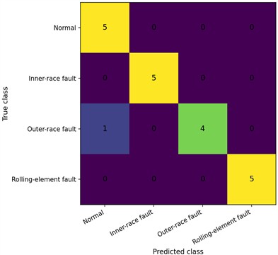
Taken together, Table 7 and Fig. 7 show that the complete model achieves high overall accuracy while also correctly identifying all held-out inner-race and rolling-element fault windows in the reported runs. As discussed in Section 4.2, the rolling-element fault record is close to the normal record in several amplitude-related statistics, yet the learned joint representation can still separate the current held-out samples. The remaining error mainly involves an outer-race fault window being predicted as normal. Section 4.3.3 therefore further examines how channel attention, multi-scale convolution, and the fusion strategy contribute to the overall performance.

4.3.3. Component ablation and amplitude-treatment controls

The preceding experiments compare the overall and class-wise performance of the complete model. To examine the effects of specific architectural choices, this section modifies the attention modules, multi-scale convolution, and fusion strategy while retaining the two-branch framework, and also includes the amplitude-treatment controls described in Section 2.3. Each configuration is independently trained using the same data partition and training protocol. The results are summarized in Table 8.

As shown in Table 8, removing temporal attention or time-frequency attention individually reduces the mean accuracy to 95.00 %. Removing all attention modules yields an accuracy of 95.00 % and a Macro-F1 of 0.9484, both below the 98.33 % accuracy and 0.9832 Macro-F1 of the complete model. Because these configurations retain both feature branches, this comparison indicates that channel attention contributes additional performance beyond the use of two branches alone. Replacing the multi-scale image convolution with a single 3×3 convolution reduces the mean accuracy to 91.67 %, while replacing feature concatenation with mean fusion yields 96.67 %. These results support the combined use of multi-scale convolution and concatenation-based fusion in the complete architecture.

Table 8Results of component ablation and amplitude-treatment control experiments

Model configuration	Accuracy (%)	Macro-F1	Parameters
Complete dual-branch model	98.33±2.89	0.9832±0.0292	1,358,732
Without temporal attention	95.00±0.00	0.9495±0.0000	1,358,604
Without time-frequency attention	95.00±0.00	0.9495±0.0000	1,337,772
Without all attention modules	95.00±5.00	0.9484±0.0521	1,337,644
Single 3 × 3 image convolution	91.67±5.77	0.9114±0.0660	1,207,052
Mean fusion instead of concatenation	96.67±2.89	0.9663±0.0292	1,358,220
Temporal z-score using training statistics	98.33±2.89	0.9832±0.0292	1,358,732
Additional log-RMS and log-PTP	93.33±2.89	0.9316±0.0310	1,358,740
Note: Values are the mean $\pm$ sample standard deviation over three random seeds, and every run uses the same 20 held-out windows. Removing time-frequency attention means removing both channel-attention modules in the CNN branch. The two amplitude-treatment controls keep the CWT image input unchanged

For amplitude treatment, temporal z-score standardization produces the same mean accuracy and Macro-F1 as per-window min-max normalization, whereas adding log-RMS and log-PTP descriptors results in a mean accuracy of 93.33 % and provides no additional benefit. The highest classification performance in the current experiment therefore does not depend on one unique temporal scaling method, and explicitly adding amplitude descriptors does not necessarily improve recognition.

Considering Tables 6 and 8 together, under the current 1200 r/min condition and fixed evaluation partition, the complete dual-branch model achieves the highest mean accuracy and Macro-F1 among the listed baselines and structural ablations and ties with its temporal z-score variant for the highest classification level among all tested configurations. The results provide complementary evidence for the branch combination and component configuration, while the associated performance-complexity trade-off is discussed in the next subsection.

4.3.4. Integrated discussion

The signal analysis in Section 4.2 and the classification experiments in Section 4.3 show that the four bearing states exhibit different behaviors in time-domain amplitude, frequency composition, and time-frequency texture, while no single representation fully separates all fault types. In particular, the rolling-element fault is close to the normal state in several time-domain indicators, including RMS and excess kurtosis, yet still exhibits localized differences in the spectrum and time-frequency distribution. This motivates the use of a TCN to encode local temporal structure in the one-dimensional vibration window, a multi-scale CNN to extract time-frequency textures from the CWT image, and channel attention to recalibrate the two feature streams before fusion.

The complete dual-branch model achieves a mean accuracy of 98.33 %±2.89 % and a Macro-F1 of 0.9832±0.0292, the highest mean classification performance among the models listed in Table 6. Its accuracy is 8.33 percentage points higher than that of the time-frequency-only branch and 5.00 percentage points higher than that of RF, indicating that the temporal and time-frequency representations provide complementary information under the present setting. The ablation results further show that removing attention reduces the mean accuracy to 95.00 %, replacing multi-scale convolution with a single-scale convolution reduces it to 91.67 %, and replacing concatenation with mean fusion results in 96.67 %. The combined architecture therefore benefits from attention, multi-scale extraction, and feature concatenation.

The complete model contains 1,358,732 trainable parameters and requires approximately 4.13 ms for a single-sample forward pass in the current CPU-based evaluation environment. This timing measures model inference after preprocessing and does not include CWT generation or data I/O. Compared with the time-frequency-only branch, the complete model introduces additional complexity but achieves higher classification performance. Thus, under the present within-record evaluation at 1200 r/min, the proposed model provides a favorable balance between classification performance and computational cost. Nevertheless, the current evidence is based on a limited number of source records, and generalization should be further examined using independent bearings and additional speed and load conditions.

5. Conclusions

This study develops a channel-attention-based TCN-CNN time-frequency dual-branch model to address the difficulty of jointly exploiting temporal and time-frequency information in bearing vibration signals from warehouse logistics sorting equipment. The TCN branch extracts local temporal features, while the CNN branch uses multi-scale convolution to learn CWT time-frequency textures; branch-specific channel attention and feature concatenation are then used for joint classification. Under the fixed 1200 r/min data partition, the proposed model achieves a mean accuracy of 98.33 %±2.89 % and a Macro-F1 of 0.9832±0.0292, the highest mean classification performance among the listed baselines. The ablation results further show that removing attention, replacing multi-scale convolution, or changing the fusion strategy reduces the classification metrics, supporting the positive role of the dual-branch representation, channel attention, and multi-scale feature extraction in the current task.

The present evaluation uses four unloaded source records at 1200 r/min and therefore remains limited in terms of independent acquisition scale. The later-stage validation behavior also indicates room for improving model regularization. Future work should first expand the dataset with independently identified bearings and clearly documented defect information to assess performance on previously unseen specimens, and then extend the evaluation to different loads, rotational speeds, and noise conditions. Further work will also investigate lightweight alternatives to the high-dimensional fully connected mapping in the time-frequency branch and complete end-to-end timing that includes preprocessing, with the aim of supporting continuous bearing-condition monitoring in sorting equipment. At the present stage, the proposed method provides an experimentally supported diagnostic framework, while its value for field deployment and maintenance decision-making requires further validation.

References

B. Feng and Q. Ye, “Operations management of smart logistics: A literature review and future research,” Frontiers of Engineering Management, Vol. 8, No. 3, pp. 344–355, Apr. 2021, https://doi.org/10.1007/s42524-021-0156-2

Publisher
Q. X. Bo et al., “Design of goods inbound and outbound strategy for automated cigarette finished-product stereoscopic warehouse,” (in Chinese), Tobacco Science and Technology, Vol. 57, No. 6, pp. 92–98, 2024, https://doi.org/10.16135/j.issn1002-0861.2024.0173

Publisher
R. B. Randall and J. Antoni, “Rolling element bearing diagnostics-A tutorial,” Mechanical Systems and Signal Processing, Vol. 25, No. 2, pp. 485–520, Nov. 2010, https://doi.org/10.1016/j.ymssp.2010.07.017

Publisher
Z. K. Peng and F. L. Chu, “Application of the wavelet transform in machine condition monitoring and fault diagnostics: A review with bibliography,” Mechanical Systems and Signal Processing, Vol. 18, No. 2, pp. 199–221, Jul. 2003, https://doi.org/10.1016/s0888-3270(03)00075-x

Publisher
R. Yan, R. X. Gao, and X. Chen, “Wavelets for fault diagnosis of rotary machines: A review with applications,” Signal Processing, Vol. 96, pp. 1–15, Apr. 2013, https://doi.org/10.1016/j.sigpro.2013.04.015

Publisher
W. Zhang, G. Peng, C. Li, Y. Chen, and Z. Zhang, “A new deep learning model for fault diagnosis with good anti-noise and domain adaptation ability on raw vibration signals,” Sensors, Vol. 17, No. 2, p. 425, Feb. 2017, https://doi.org/10.3390/s17020425

Publisher
D.-T. Hoang and H.-J. Kang, “Rolling element bearing fault diagnosis using convolutional neural network and vibration image,” Cognitive Systems Research, Vol. 53, pp. 42–50, Mar. 2018, https://doi.org/10.1016/j.cogsys.2018.03.002

Publisher
R. Zhao, R. Yan, Z. Chen, K. Mao, P. Wang, and R. X. Gao, “Deep learning and its applications to machine health monitoring,” Mechanical Systems and Signal Processing, Vol. 115, pp. 213–237, Jun. 2018, https://doi.org/10.1016/j.ymssp.2018.05.050

Publisher
Y. Lei, B. Yang, X. Jiang, F. Jia, N. Li, and A. K. Nandi, “Applications of machine learning to machine fault diagnosis: A review and roadmap,” Mechanical Systems and Signal Processing, Vol. 138, p. 106587, Jan. 2020, https://doi.org/10.1016/j.ymssp.2019.106587

Publisher
S. Xiong, L. Zhang, Y. Yang, H. Zhou, and L. Zhang, “Multi-source information-based bearing fault diagnosis using multi-branch selective fusion deep residual network,” Sensors, Vol. 24, No. 20, p. 6581, Oct. 2024, https://doi.org/10.3390/s24206581

Publisher
J. Yasenjiang, Y. Zhao, Y. Xiao, H. Hao, Z. Gong, and S. Han, “Bearing fault diagnosis based on time-frequency dual domains and feature fusion of ResNet-CACNN-BiGRU-SDPA,” Sensors, Vol. 25, No. 13, p. 3871, Jun. 2025, https://doi.org/10.3390/s25133871

Publisher
Q. Liu, M. Chen, M. Tang, and H. Lai, “A bearing fault diagnosis method based on an attention mechanism and a dual-branch parallel network,” Applied Sciences, Vol. 16, No. 9, p. 4511, May 2026, https://doi.org/10.3390/app16094511

Publisher
J. Hu, L. Shen, and G. Sun, “Squeeze-and-Excitation Networks,” in IEEE/CVF Conference on Computer Vision and Pattern Recognition, pp. 7132–7141, 2018, https://doi.org/10.1109/cvpr.2018.00745

Publisher
S. Woo, J. Park, J.-Y. Lee, and I. S. Kweon, “CBAM: Convolutional block attention module,” in Lecture Notes in Computer Science, Cham: Springer International Publishing, 2018, pp. 3–19, https://doi.org/10.1007/978-3-030-01234-2_1

Publisher
W. Wei and Y. Yuan, “VMD-DCA-BiGRU wind turbine bearing fault diagnosis method with attention mechanism integration,” Measurement, Vol. 266, p. 120466, Jan. 2026, https://doi.org/10.1016/j.measurement.2026.120466

Publisher
N. Rezazadeh, F. Caputo, A. Aversano, G. Lamanna, A. de Luca, and D. Perfetto, “Prototype-attention domain adaptation for explainable bearing fault diagnosis,” Procedia Structural Integrity, Vol. 80, pp. 411–417, 2026, https://doi.org/10.1016/j.prostr.2026.02.039

Publisher

About this article

Received

July 8, 2026

Accepted

September 22, 2026

Published

October 30, 2026

SUBJECTS

Fault diagnosis based on vibration signal analysis

DOI

https://doi.org/10.21595/jve.2026.26815

Keywords

warehouse logistics sorting machine

bearing fault diagnosis

time-frequency dual-branch network

channel attention

predictive maintenance

Acknowledgements

The authors have not disclosed any funding.

Data Availability

The datasets generated during and/or analyzed during the current study are available from the corresponding author on reasonable request.

Author Contributions

Changhua Chen: conceptualization, research design, methodology guidance, validation, and writing. Xiangyang Deng: methodology, software implementation, data preprocessing, model construction, formal analysis, visualization, and experimental validation. Xinqi Wan: data acquisition, signal processing, comparative experimental analysis, and result interpretation.

Conflict of interest

The authors declare that they have no conflict of interest.

This is an open access article distributed under the Creative Commons Attribution License (CC BY 4.0), which permits unrestricted use, distribution, and reproduction in any medium, provided the original work is properly cited.

C. Chen, X. Deng, and X. Wan, “Channel-attention-based time-frequency dual-branch network for bearing fault diagnosis in warehouse logistics sorting machines,” Journal of Vibroengineering, Vol. 28, No. 8, –20, Oct. 2026, https://doi.org/10.21595/jve.2026.26815

Copy Extrica

Copied to clipboard!

TY  - JOUR
DO  - 10.21595/jve.2026.26815
UR  - https://doi.org/10.21595/jve.2026.26815
TI  - Channel-attention-based time-frequency dual-branch network for bearing fault diagnosis in warehouse logistics sorting machines
T2  - Journal of Vibroengineering
AU  - Chen, Changhua
AU  - Deng, Xiangyang
AU  - Wan, Xinqi
PY  - 2026
DA  - 2026/10/30
PB  - Extrica
VL  - 28
IS  - 8
SN  - 1392-8716
SN  - 2538-8460
ER  - 

Copy Ris

Copied to clipboard!

@article{doi_10.21595/jve.2026.26815,
  title = {Channel-attention-based time-frequency dual-branch network for bearing fault diagnosis in warehouse logistics sorting machines},
  author = {Chen, Changhua and Deng, Xiangyang and Wan, Xinqi},
  journal = {Journal of Vibroengineering},
  year = {2026},
  month = {10},
  volume = {28},
  number = {8},
  doi = {10.21595/jve.2026.26815},
  url = {https://doi.org/10.21595/jve.2026.26815},
  publisher = {Extrica},
  issn = {1392-8716},
  eissn = {2538-8460},
}

Copy Bibtex

Copied to clipboard!

[1]C. Chen, X. Deng, and X. Wan, “Channel-attention-based time-frequency dual-branch network for bearing fault diagnosis in warehouse logistics sorting machines,” Journal of Vibroengineering, Oct. 2026, doi: 10.21595/jve.2026.26815.

Copy IEEE

Copied to clipboard!

Chen, Changhua, Xiangyang Deng, and Xinqi Wan. “Channel-attention-based time-frequency dual-branch network for bearing fault diagnosis in warehouse logistics sorting machines.” Journal of Vibroengineering 28, no. 8 (2026). https://doi.org/10.21595/jve.2026.26815.

Copy Chicago

Copied to clipboard!

Channel-attention-based time-frequency dual-branch network for bearing fault diagnosis in warehouse logistics sorting machines

Abstract

Highlights

1. Introduction

2. Data acquisition and signal preprocessing

2.1. Bearing conditions and data acquisition

2.2. Sliding-window segmentation and chronological sample partitioning

2.3. Data normalization

2.4. Continuous wavelet transform

3. Channel-attention-based time-frequency dual-branch model

3.1. Overall architecture

3.2. TCN temporal feature branch

3.3. CNN time-frequency feature branch

3.4. Channel-attention mechanism

3.4.1. Temporal channel-attention design

3.4.2. Time-frequency channel-attention design

3.5. Feature fusion and classification

3.6. Evaluation metrics

4. Experimental results and analysis

4.1. Experimental settings and comparison protocols

4.2. Bearing vibration signal characteristics

4.2.1. Time-domain characteristics

4.2.2. Frequency-domain characteristics

4.2.3. Time-frequency characteristics

4.3. Model diagnosis analysis

4.3.1. Training process and overall performance

4.3.2. Class-wise recognition and misclassification analysis

4.3.3. Component ablation and amplitude-treatment controls

4.3.4. Integrated discussion

5. Conclusions

References

About this article

Related Articles