Parametric excitation of railway car body sway induced by nonlinear air spring stiffness

1. Introduction

In recent years, with the continuous increase in train operational mileage, numerous vehicles have experienced a multitude of dynamic problems. The operational smoothness and ride comfort of these vehicles have significantly deteriorated, primarily manifesting as low-frequency car body wobble and abnormal jitter. The car body wobble is characterized by large amplitudes and long durations, with frequencies concentrated mainly between 2 and 3 Hz. Conversely, the car body jitter is of shorter duration and frequently occurs when the vehicle traverses specific track sections, causing distinct passenger discomfort, as well as noticeable shaking and anomalous noises from seats and luggage racks. Sun et al. [1] discovered that as the vehicle speed increases, the damping coefficient of the vehicle’s upper-center roll mode first increases and then decreases. Furthermore, it was observed that the damping coefficient of the car body hunting motion becomes very small due to wheel-rail mismatch. Huang et al. [2], using the root locus method, investigated the influence patterns of vehicle parameters on low-frequency lateral wobble. Their research results indicated that the occurrence of low-frequency lateral wobble can be avoided by selecting appropriate suspension parameters, wheel-rail parameters, and car body mass parameters. Wu et al. [3] established a multi-body dynamics model based on linear and nonlinear analysis, finding that under certain boundary conditions, bogie hunting motion can lead to low-frequency car body sway. This low-frequency sway phenomenon is caused by excessively low wheel-rail contact conicity or mismatched suspension parameters. Chen et al. [4], employing the Euclidean closeness criterion from fuzzy mathematics, effectively tracked and analyzed the variation of vehicle rigid-body modes with speed. He found that resonance occurs between bogie hunting motion and car body lateral motion, causing low-frequency lateral wobble of the car body. Zhou et al. [5] analyzed the impact of modal parameters from partial degrees of freedom of the vehicle system on its vertical and lateral smoothness, and analyzed the influence of secondary suspension parameters on these modal parameters, providing a basis for improving the vehicle's operational smoothness. Shi et al. [6], based on the concept of coupling degree, studied the influencing factors of the vehicle system's coupling degree. The conclusion drawn was that, within a reasonable range, increasing the damping of the secondary lateral dampers or decreasing the secondary lateral stiffness can reduce the system's coupling level and enhance vehicle smoothness. Zong et al. [7], aiming to reduce the coupling resonance between various modes of the vehicle system, employed a genetic algorithm to optimize the secondary suspension parameters. This allowed for the calculation of parameter values that minimize the coupling degree. They pointed out that secondary lateral damping and stiffness have a significant impact on the coupling degree, and adjusting these factors can mitigate the influence of bogie hunting on car body lateral motion. Xu [8] argued that the equivalent conicity must be controlled within a reasonable range; otherwise, excessively high conicity will lead to bogie hunting, while excessively low conicity will result in car body wobble. In summary, lateral wobble of the railway vehicle car body is primarily caused by resonance effects. By appropriately modifying parameters, the hunting frequency can be shifted away from the car body's natural frequency. However, in some cases, vehicles experience low-frequency lateral wobble even when operating below the critical speed, which cannot be explained by these two reasons. For instance, Liu [9] discovered severe lateral wobble at 90 km/h when the hunting frequency was far from the car body’s natural frequency. To address this issue, linear theory is no longer sufficient; the influence of nonlinear factors must be considered, specifically, the impact of internal parametric excitation within the vehicle system on car body wobble. Furthermore, most studies focus on external lateral excitation, while few explore the influence of external vertical excitation on car body lateral motion.

The high-speed train is a strongly nonlinear system [10-12], encompassing nonlinear wheel-rail contact relationships and nonlinear suspension components. Among these, air springs, possessing excellent vibration isolation performance, are widely utilized in various vehicles to enhance ride comfort. However, air spring modeling is complex and involves numerous parameters. In most vehicle dynamics calculations, air springs are merely treated as force elements consisting of a spring and a damper in parallel. While this simplified approach facilitates computation, it fails to adequately consider the influence of the air spring's internal pneumatic characteristics on the overall system performance. Gao [13] established a TPL-ASN nonlinear model for air springs, skillfully resolving the connection problem between the throttle orifice and the connecting pipe using an auxiliary space method. Li et al. [14] derived a physical model of the air spring based on fluid dynamics and thermodynamics and provided a calculation method for air spring parameters. Li [15] proposed a thermodynamic air spring modeling method that requires neither empirical determination nor experimental parameter identification. Through a PID-based height control strategy, using the solenoid valve opening as input and car body height as output, the main chamber volume was altered, achieving good control results. Liu [16] focused primarily on the vertical mechanical characteristics of air springs, obtaining the influence of the spring's own structural parameters and external excitation on its mechanical properties through extensive experimentation. Docquier [17] proposed a relatively complete thermodynamic model suitable for multi-body simulation of railway vehicles (0-20 Hz); however, this model cannot well reflect the characteristics of air springs equipped with throttle orifices and neglects the effects of temperature variation, height valves, and differential pressure valves. Wu et al. [18], based on thermodynamics and energy dissipation theory, proposed a dynamic stiffness model for vehicular air springs that considers equivalent damping and hysteretic characteristics. This model does not impose restrictions on the gas exchange process within the air spring, thus offering a degree of general applicability. Liu and Lee [19] focused on the dynamic stiffness and overall equivalent damping of air springs connected to throttle orifices and auxiliary reservoirs. Utilizing the energy conservation equation, the equation of state for gas, and the orifice flow equation, they derived a theoretical model for the air spring and its auxiliary reservoir. Chen et al. [20], from a geometric analysis perspective, used the arc length of the air spring's rubber bellows and the effective radii of the upper and lower plates as design variables to derive a mathematical prediction model for the structural parameters of bellows-type air springs. They established a unified vertical stiffness model that incorporates structural parameters and the stiffness of the rubber bellows. Ouyang et al. [21] investigated the nonlinear mechanical properties of air springs, studying their geometric structure and shape deformation characteristics. They employed numerical calculation methods to determine the air spring's volume variation and presented the relationship curves between the force and displacement of the air spring. Zhao et al. [22], addressing the significant discrepancy between the actual and theoretical stiffness of air springs, established an improved stiffness model for constrained membrane-type air springs, wherein the rate of change of the effective area and the rate of change of the effective volume were derived entirely through geometric deduction. Zhang et al. [23] established a vertical nonlinear dynamic model of an air spring system and a dynamic model of a specific high-speed train. They validated the accuracy of the nonlinear air spring dynamic model based on the results of air spring vertical vibration transmission tests. In summary, although extensive research has been conducted on air spring modeling to date, vehicle dynamics models that account for the nonlinear characteristics of air springs are not commonly found.

For the study of nonlinear dynamic systems, the primary methods include perturbation methods, the harmonic balance method, the averaging method, the method of multiple scales, and asymptotic methods, among others [24-25]. Among these, the method of multiple scales (MMS) is a classic and widely applied technique. It is applicable not only to strictly periodic motion but also to the decaying vibrations of dissipative systems and non-steady-state processes [26]. In the 1950s, Sturrock first proposed the method of multiple scales. Subsequently, Nayfeh and Mook [27] further developed and refined this method. Numerous scholars have since employed this method to analyze the dynamic responses of nonlinear systems. Du and Li [28] and Feng et al. [29] utilized the method of multiple scales to discuss the nonlinear vibration of marine rotary machinery-airbag isolation systems and the nonlinear harmonic resonance problem of vibrating screens, respectively, and verified the correctness of the MMS analysis. Qian et al. [30] combined the method of multiple scales with numerical simulations to conduct a nonlinear dynamic analysis of the vortex-induced vibration f cables featuring 2:1 internal resonance; their work revealed the influence of structural and aerodynamic parameters on the "lock-in" domain and the jump phenomenon. Binatari et al. [31] proposed a method of multiple scales suitable for delay differential equations; by considering all roots of the characteristic equation and the initial conditions over an interval, they achieved high-precision approximate solutions over long-time scales. Li et al. [32-33] used the method of multiple scales to analyze the combined principal-super harmonic and principal-subharmonic resonances in a Duffing system. Currently, the method of multiple scales has broad applications, covering multiple fields from basic science to engineering technology. This paper considers the nonlinear characteristics of a certain component within the vehicle system to investigate the phenomenon of parametrically excited vibration in the vehicle system.

2. Modelling

2.1. Air spring model

Referencing [21], a vertical dynamic model of the air spring is established based on air thermodynamics, as shown in Fig. 1, with parameters listed in Table 1. The model, which considers gas flow and the thermodynamic state of the air, is primarily composed of the main air spring chamber, an auxiliary.

Fig. 1Air spring model

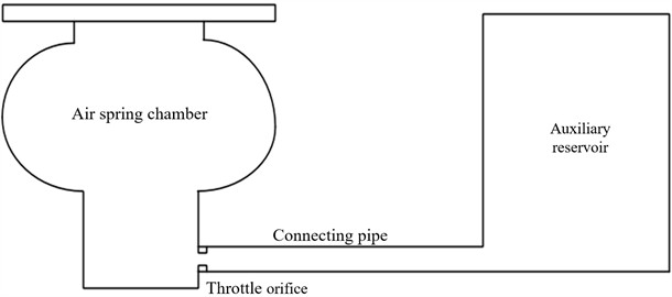
Table 1Basic parameters of the air spring model

Parameter	Value	Unit
Air spring main chamber volume	55	L
Air spring auxiliary reservoir volume	220	L
Air spring effective area	0.2	m2
Rate of change of air spring effective area	0.06	m2/m
Pipe diameter	0.055	m
Pipe length	0.065	m
Throttle orifice diameter	0.014	m
Ambient temperature	293	K
Heat transfer coefficient	200	W/(m2·K)
Polytropic exponent of gas	1.32	–

The pressure in the main air spring chamber satisfies the polytropic gas equation:

1

${\dot{p}}_{asb}=\frac{1}{V_{asb}^n}\left({\dot{m}}_{asb}R{T}_{asb}+m_{asb}R{\dot{T}}_{asb}-n{p}_{asb}{V}_{asb}^{n-1}{\dot{V}}_{asb}\right),$

where: $p_{asb}$ is the gas pressure in the main air spring chamber; $V_{asb}$ is the volume of the main air spring chamber; $m_{asb}$ is the mass of the gas within the main chamber; $R$ is the thermodynamic gas constant; $T_{asb}$ is the gas temperature within the main chamber; and $n$ is the polytropic exponent of the gas. Since the volume of the auxiliary reservoir $V_{asf}$ remains constant during operation, the pressure within the auxiliary reservoir satisfies:

2

${\dot{p}}_{asf}=\frac{1}{V_{asf}^n}\left({\dot{m}}_{asf}R{T}_{asf}+m_{asf}R{\dot{T}}_{asf}\right),$

where: $p_{asf}$ is the gas pressure within the auxiliary reservoir; $m_{asf}$ is the mass of the gas within the auxiliary reservoir; $T_{asf}$ is the gas temperature within the auxiliary reservoir. The vertical force $F_{asz}$ exerted by the air spring on the car body is:

3

$F_{asz}=\left(A_0+\frac{d{A}_0}{dz}z\right)p_b,$

where: $A_0$ is the static load-bearing area of the air spring; $d{A}_0/dz$ is the rate of change of the air spring’s load-bearing area with respect to the vertical height $z$. A throttle orifice can be installed between the main air spring chamber and the auxiliary reservoir. As air flows through the orifice, a portion of the vibration energy is dissipated due to resistance, thereby achieving a damping effect. Based on the theories of fluid dynamics and air thermodynamics, the mass flow rate $Q$ of the gas passing through the throttle orifice can be expressed as:

When $p_d/p_u\le 0.546$:

4

$Q=C_{q}A{p}_u\sqrt{\frac{\mu }{R{T}_u}{\left(\frac{2}{\mu +1}\right)}^{\frac{\mu +1}{\mu -1}}}.$

When $\frac{p_d}{p_u}>0.546$:

5

$Q=C_{q}A{p}_u\sqrt{\frac{2\mu }{R{T}_u\left(\mu -1\right)}\left[{\left(\frac{p_d}{p_u}\right)}^{\frac{2}{\mu }}-{\left(\frac{p_d}{p_u}\right)}^{\frac{\mu +1}{\mu }}\right]},$

6

$C_q=0.8414-0.1002\left(\frac{p_d}{p_u}\right)+0.8415{\left(\frac{p_d}{p_u}\right)}^2-3.9{\left(\frac{p_d}{p_u}\right)}^3+\mathrm{4.60010.8415}{\left(\frac{p_d}{p_u}\right)}^4-1.6827{\left(\frac{p_d}{p_u}\right)}^5,$

where: $C_q$ is the flow coefficient of the throttle orifice; 0.546 is the critical pressure ratio across the orifice; $\mu$ is the isentropic exponent (ratio of specific heats) of the gas; $p_d$ and $p_u$ are the absolute pressures of the gas in the downstream and upstream chambers, respectively; $T_u$ is the temperature of the gas in the upstream chamber; and $A$ is the flow area of the throttle orifice. When an external excitation acts on the air spring surface, causing its vertical height to change, the effective area and effective volume of the air spring change accordingly. According to the polytropic gas equation, this affects the pressures within the main air spring chamber and the auxiliary reservoir. When the pressures in the main chamber and the auxiliary reservoir fail to reach dynamic equilibrium, gas is exchanged between the two chambers through the throttle orifice. During this process, the vertical force $F_z$ exerted by the air spring on the car body is constantly changing.

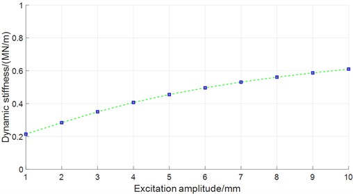
Based on the simulation results, it is found that the stiffness of the air spring varies with the external excitation frequency. This variation trend is illustrated in Fig. 2: in the frequency ranges of 0-0.3 Hz and 1.5-3 Hz, the change in dynamic stiffness is relatively small, whereas in the frequency range of 0.3-1.5 Hz, the dynamic stiffness changes significantly. As shown in Fig. 3, for the same excitation frequency of 1 Hz, the magnitude of the dynamic stiffness also differs with varying excitation amplitudes.

Fig. 2Effect of excitation frequency on dynamic stiffness

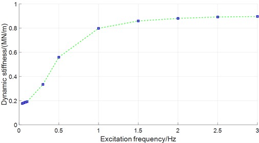
Fig. 3Effect of excitation amplitude on dynamic stiffness

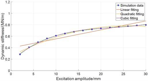
Based on the analysis above, the dynamic stiffness of the air spring does not change significantly when the excitation frequency is greater than 2 Hz. Selecting an excitation frequency of 2 Hz, a polynomial fit is performed on the dynamic stiffness of the air spring under different amplitudes; the fitting results are shown in Fig. 4. The higher the order of the selected fitting polynomial, the better the fitting effect. However, increasing the polynomial order will also increase the complexity of subsequent dynamic modeling and vibration analysis. To balance model accuracy and computational efficiency, a quadratic polynomial is ultimately chosen to describe the nonlinear stiffness characteristics of the air spring. Thus, the vertical stiffness of the air spring can be expressed as:

7

$a\cdot x^2+k_z\cdot x+a_0,$

where: $a_0=$ 0.2526, $a=$ 0.0413, $k_z=$ –0.0008.

Fig. 4Results of data fitting

2.2. 3-DOF vehicle model

A 3-degree-of-freedom (3-DOF) vehicle model, incorporating the car body’s bounce motion ($z_c$), roll motion (${\theta }_c$), and lateral motion ($y_c$), is established using the vertical vibration of the bogie frame as the input, as shown in Fig. 5. The vehicle parameters are provided in Table 2. When relative displacements and relative velocities are generated between the various components of the vehicle system, the suspension system produces forces and moments. If the deformation of each component were to be precisely considered, the expressions for the secondary suspension forces would become highly complex. Consequently, this paper only considers the nonlinearity of the air spring’s vertical force, while neglecting the nonlinearity of the air spring’s lateral force and the series stiffness of the dampers.

Fig. 53-DOF vehicle model

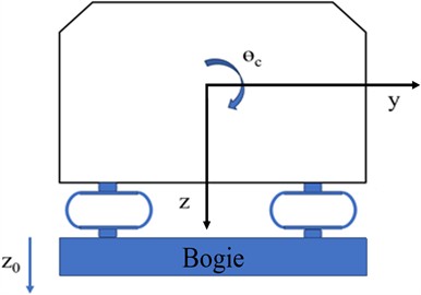
Table 23-DOF vehicle model

Parameter	Symbol	Value	Unit
Mass of vehicle	$M_c$	56000	kg
Roll moment of inertia	$J_{cx}$	110000	kg·m2
Height from car body gravity center to the suspension	$h$	0.6	m
Half of the lateral span of secondary suspension	$b$	1	m
Lateral stiffness of air spring	$k_y$	0.15	MN/m
Lateral damping of secondary suspension	$c_y$	0.2	kN·s/m
Vertical damping of secondary suspension	$c_z$	10	kN·s/m
Stiffness of anti-roll torsion bar	$K$	2	MN·m/rad

The secondary suspension adopts a spring-damper parallel model. The expressions for each force element and the equations of motion for each DOF of the car body are as follows:

Secondary vertical force:

8

$\left\{\begin{array}{c}{F}_{zl}=k_z\left(z_c-z_0-{\theta }_{c}b\right)+a{\left(z_c-z_0-{\theta }_{c}b\right)}^2+c_z\left({\dot{z}}_c-{\dot{z}}_0-{\dot{\theta }}_{c}b\right),\\ F_{zr}=k_z\left(z_c-z_0+{\theta }_{c}b\right)+a{\left(z_c-z_0+{\theta }_{c}b\right)}^2+c_z\left({\dot{z}}_c-{\dot{z}}_0+{\dot{\theta }}_{c}b\right).\end{array}\right.$

Secondary lateral force:

9

$F_y=k_y\left(y_c-{\theta }_{c}h\right)+c_y\left({\dot{y}}_c-{\dot{\theta }}_{c}h\right).$

Car body bounce motion equation:

10

$M_c{\ddot{z}}_c+2F_{zl}+2F_{zr}=0.$

Car body lateral motion equation:

11

$M_c{\ddot{y}}_c+4F_y=0.$

Car body roll motion equation:

12

$J_{cx}{\ddot{\theta }}_c-2F_{zl}b+2F_{zr}b-4F_{y}h-M_{c}g{\theta }_{c}h+2K{\theta }_c=0.$

Substituting Eq. (8) and Eq. (9) into Eqs. (10-12) respectively, and simplifying, the 3-DOF car body vibration equations can be obtained as:

13

$\left\{\begin{array}{l}{M}_c{\ddot{z}}_c+4c_z\left({\dot{z}}_c-{\dot{z}}_0\right)+4k_z\left(z_c-z_0\right)+4a{\left(z_c-z_0\right)}^2+4a{b}^2{\theta }_c^2=0,\\ M_c{\ddot{y}}_c+4c_y\left({\dot{y}}_c-{\dot{\theta }}_{c}h\right)+4k_y\left(y_c-{\theta }_{c}h\right)=0,\\ J_{cx}{\ddot{\theta }}_c+\left(4c_z{b}^2+4c_y{h}^2\right){\dot{\theta }}_c+\left(4k_z{b}^2+4k_y{h}^2-M_{c}gh+2K\right){\theta }_c\\ +8a{b}^2\left(z_c-z_0\right){\theta }_c-4k_{y}h{y}_c-4c_{y}h{\dot{y}}_c=0.\end{array}\right.$

3. Analytical solution

The lateral motion and roll motion of the car body are coupled with each other. When the lateral motion and roll motion are in phase, it forms the car body’s lower-center sway motion; when the lateral motion and roll motion are out of phase, it forms the car body’s upper-center sway. When the car body sways, the sway radius is a constant value. Introducing the sway radius, let $z=z_c-z_0$ and substitute it into Eq. (13). When the car body undergoes lower-center sway, let the sway radius be $R_1$, then Eq. (13) can be simplified to:

When the car body undergoes upper-center sway, let the sway radius be $R_2$, then Eq. (13) can be simplified to:

Using the method of multiple scales to solve the above equations, and taking the car body’s lower-center sway as an example, the simplified system equation can be obtained as:

where:

The first expression in Eq. (16) represents a forced vibration process. The car body bounce response frequency matches the external excitation frequency. Let:

where $A$ is the amplitude of the car body bounce response, and $\omega$ is the external excitation frequency. Substitute Eq. (17) into Eq. (16). To simplify the analysis, the influence of damping is neglected. Damping affects the critical threshold for the occurrence of coupled vibration, but it does not affect the mechanism of the system's nonlinear coupling. This gives:

When the external excitation frequency is close to the car body bounce frequency, i.e., $\omega \approx {\omega }_1$, let $F={\epsilon }^{2}f$, $\omega \approx {\omega }_1+\epsilon {\sigma }_1$. To make the damping effect and the nonlinear effect appear in the same perturbation equation, let:

where $\epsilon$ is a small parameter, taken as 0.1. Assume the solution is:

where $T_n={\epsilon }^{n}t$. Substitute Eq. (20) into Eq. (16), and let the coefficients of the same powers of $\epsilon$ be equal, yielding:

The general solution to Eq. (21) is:

Substitute Eq. (23) into Eq. (22) and rearrange to get:

When the car body bounce frequency is far from 2 times the roll frequency, i.e., ${\omega }_1$ is far from ${\omega }_2$, the secular terms are independent of nonlinear factors. Eliminating the secular terms from Eq. (24) and Eq. (25) gives:

where ${\gamma }_1={\sigma }_1{T}_1+\theta -{\beta }_1$. For the steady-state response:

Substituting Eq. (28) into Eqs. (26-27) yields the solution:

Substituting Eq. (29) into Eq. (16), the steady-state solution to Eq. (10) can be obtained as:

where ${\gamma }_1=-\text{arctg}\left({\mu }_1/{\sigma }_1\right)$. The above shows that at the first approximation, the solution is not affected by nonlinear factors; it is, in fact, the solution for the linear system. When the car body bounce frequency is close to 2 times the roll frequency, i.e., ${\omega }_1\approx 2{\omega }_2$, let:

Then, $\cos \left(2{\omega }_2{T}_0+2{\beta }_2\right)$ in Eq. (24) and $\cos \left[\left({\omega }_1-{\omega }_2\right)T_0+{\beta }_1-{\beta }_2\right]$ in Eq. (25) will also produce secular terms. Eliminating the secular terms yields:

where ${\gamma }_2={\sigma }_2{T}_1+{\beta }_1-2{\beta }_2$. For the steady-state response:

Substituting Eq. (34) into Eq. (32) and Eq. (33), there are two possible solutions. One solution is Eq. (30), and the other is:

where:

Substituting Eq. (35) into Eq. (20), the steady-state solution to Eq. (16) can be obtained as:

When $f<\frac{{\alpha }_2{P}_2}{2}$, the solution is unique. When $f<\frac{{\alpha }_2\sqrt{P_1^2+P_2^2}}{2}$, there are two possible solutions. When $\frac{{\alpha }_2{P}_2}{2}<f<\frac{{\alpha }_2\sqrt{P_1^2+P_2^2}}{2}$ and $P_1<0$, there are three possible solutions. If ${\sigma }_1={\sigma }_2=0$, the minimum excitation value required to incite the car body’s lower-center sway is:

Fig. 6Response amplitude vs. excitation amplitude

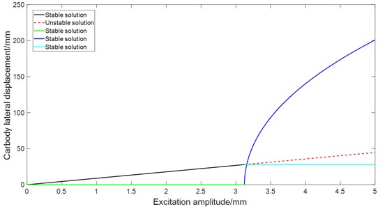
When the external excitation frequency is equal to the bounce natural frequency, i.e., ${\sigma }_1=0$, and the vehicle parameters are substituted into the steady-state solution Eq. (38), the results are shown in Fig. 6. When the bounce motion amplitude of the bogie frame exceeds 3.1 mm, the lateral motion of the car body is excited. As the excitation continuously increases, the amplitude of the car body's lateral motion gradually increases, while the relative motion amplitude between the car body and the bogie frame in the bounce direction remains constant, exhibiting a saturation phenomenon.

4. Numerical solution

To ensure the feasibility of the analytical solution, the influence of damping effects was neglected during the mechanism analysis phase. In order to investigate the dynamic evolution process of the car body vibration response more accurately under actual operating conditions, this paper employs the fourth-order Runge-Kutta method, based on the MATLAB platform, to numerically solve the system equations for the 3-DOF nonlinear model and validate the accuracy of the analytical method.

A simulation is conducted with the external excitation amplitude set to 4.5 mm. As shown in Figs. 7-9, The time-domain results clearly reveal the internal energy transfer mechanism within the system: the response is initially dominated by the bounce motion, but as time progresses, the roll and lateral motions are gradually excited. This process is accompanied by a decrease in the bounce motion amplitude and an increase in the amplitudes of the roll and lateral motions, all of which eventually converge to a steady state. This phenomenon indicates that, due to the influence of nonlinear coupling factors, energy has permeated from the bounce motion mode to the other two motion modes.

Fig. 7Response amplitude vs. excitation frequency

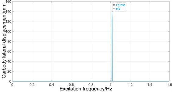
Fig. 8Response amplitude vs. excitation amplitude

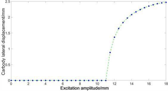
Fig. 9Numerical solution of vehicle vibration response

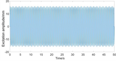
a) Wheel-rail excitation

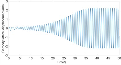
b) Car body lateral motion

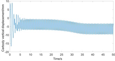
c) Car body vertical motion

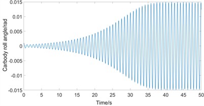
d) Car body roll motion

5. Comparative analysis with a 10-DOF vehicle model

In the 3-DOF model, the influence of excitation phase difference on vehicle vibration was not considered. Assume a train is operating on a track, and the train is perfectly symmetrical front-to-back and left-to-right. When the vehicle runs on a corrugated (sinusoidal) track, the vertical displacements of the 1st, 2nd, 3rd, and 4th wheelsets are $z_{01}$, $z_{02}$, $z_{03}$, and $z_{04}$ respectively. Their expressions can be written as:

where:

where, $a_0$ is the vertical amplitude of the track, $\omega$ is the track excitation frequency, $L_r$ is the wavelength of the track, $v$ is the vehicle operating speed, ${\beta }_1$ is the phase lag of the second wheelset relative to the first, ${\beta }_2$ is the phase lag of the third wheelset relative to the first, and ${\beta }_3$ is the phase lag of the fourth wheelset relative to the first. The bounce and lateral motions of the front and rear bogies are $z_1$ and $z_2$, and $y_1$ and $y_2$, respectively; their pitch motions are ${\phi }_1$ and ${\phi }_2$. The bounce motion of the car body is $z_3$, lateral motion is $y_3$, roll motion is ${\theta }_3$, and pitch motion is ${\phi }_3$. The full-vehicle model is shown in Fig. 10. The vehicle parameters are provided in Table 3.

The primary and secondary suspensions adopt a spring-damper parallel model. The expressions for each force element and the equations of motion for each DOF of the vehicle model are as follows.

Bogie primary vertical force is:

Bogie primary lateral force is:

Bogie primary longitudinal force is:

Secondary vertical force is:

Secondary lateral force is:

Secondary longitudinal force is:

Bogie 1 bounce motion is:

Bogie 1 lateral motion is:

Bogie 1 pitch motion is:

Bogie 2 bounce motion is:

Bogie 2 lateral motion is:

Bogie 2 pitch motion is:

Car body bounce motion is:

Car body lateral motion is:

Car body pitch motion is:

Car body roll motion is:

The vehicle operating speed is selected as 250 km/h to compare the difference in vibration response between the 3-degree-of-freedom model and the 10-degree-of-freedom model under the same excitation frequency and amplitude. With the track excitation frequency and vehicle operating speed known, the track wavelength is 28.74 m.

When the excitation frequency is 2.5 Hz and the excitation amplitude is 20 mm, the vibration responses of the half-car model and the full-car model are shown in Fig. 11. Under the same excitation conditions, the lateral vibration of the car body in the half-car model (3-DOF model) is excited, whereas the lateral vibration of the car body in the full-car model (10-DOF model) gradually attenuates. By comparing the bounce motions of the bogie frames and the car body in both models, it is found that the main reason for this phenomenon is that the 1st and 2nd bogies in the full-car model do not vibrate synchronously and have a phase difference, which weakens the amplitude of the car body’s bounce motion.

Fig. 1010-DOF vehicle model

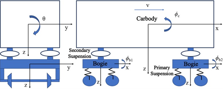
Fig. 11Comparison of 3-DOF results with 10-DOF results

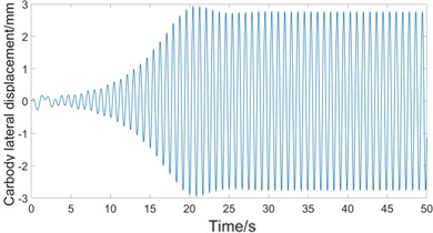
a) 3-DOF lateral motion

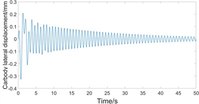
b) 10-DOF lateral motion

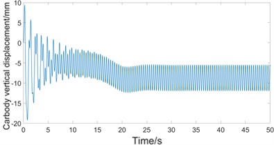
c) 3-DOF vertical motion

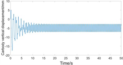
d) 10-DOF vertical motion

6. Conclusions

In this paper, a vertical dynamic model of the air spring was established based on air thermodynamics, and a quadratic polynomial was used to describe the nonlinear relationship between its supporting reaction force and the excitation amplitude. Building upon this foundation, a 3-DOF vehicle dynamics model was established and solved using both the method of multiple scales and numerical methods, leading to the following conclusions:

1) The numerical calculation results demonstrate that when the frequency of the bogie frame’s vertical excitation is approximately twice the natural frequency of the system’s upper-center sway or lower-center sway, the corresponding car body sway motion will be excited.

2) The lateral motion is triggered only when the bounce amplitude of the bogie frame exceeds a critical threshold of 3.1 mm. This critical threshold is related to the vehicle's structural and suspension parameters, and its magnitude is positively correlated with the secondary suspension damping and the natural frequency of the vehicle system’s sway motion. Furthermore, the car body’s lower-center roll/sway motion is only excited when the secondary lateral damping is small. Because the frequency band that excites the vehicle's parametric resonance is narrow, the phenomenon can be avoided by modifying the vehicle's structural or suspension parameters.

3) The wheel-rail excitation frequency is related to the track wavelength and the vehicle operating speed. For a specific track wavelength, the vehicle's parametric resonance phenomenon can only be excited within a certain speed range. Moreover, the track wavelength will cause a phase difference between different wheelsets, which has an attenuation effect on the car body's vertical vibration.