Abstract
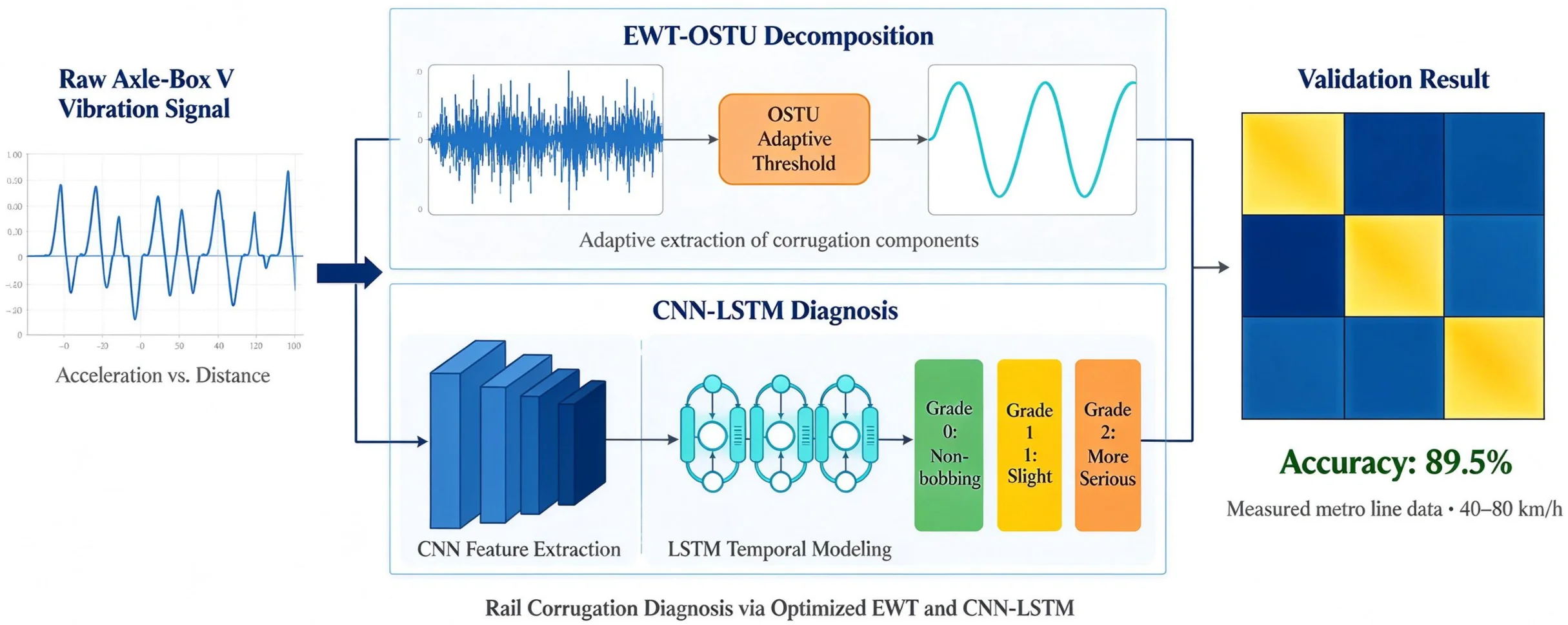
Rail corrugation is a common short-wave defect of metro rails that can excite strong wheel-rail vibration and compromise running safety and ride quality. Its efficient identification from axle box vibration signals remains challenging because weak corrugation components are easily masked by wheel-rail noise, and conventional fixed-threshold decomposition methods cannot adapt to varying operating conditions. To fill this gap, this paper optimizes the empirical wavelet transform (EWT) using the Otsu maximum between-class variance method (OSTU) to extract corrugation features adaptively from axle box signals, and proposes a CNN-LSTM intelligent diagnosis model for rail corrugation. A wheel–rail coupled dynamic model is established and a simulation method of rail corrugation is given; simulation validation shows that the decomposition algorithm can effectively separate corrugation components and reduce the influence of the preset threshold. The model is then experimentally validated on actual line data measured on an operating metro line, achieving a diagnostic accuracy of 89.5 % on the test set and demonstrating good performance across all corrugation grades.
Highlights
- A CNN-LSTM intelligent diagnosis model integrates convolutional spatial feature extraction with LSTM temporal dependency modeling, enabling automatic multi-grade classification of rail corrugation severity without hand-crafted features.
- Validated on measured metro line data across 40–80 km/h, the model achieves 89.5% overall diagnostic accuracy, with zero misclassification between healthy (Grade 0) and severely corrugated (Grade 2) track sections.
- An OSTU-optimized empirical wavelet transform (EWT-OSTU) is proposed to adaptively extract rail corrugation components from axle-box vibration signals, eliminating reliance on fixed decomposition thresholds that cannot adapt to varying operating conditions.
- A wheel-rail coupled dynamics model is established and validated through co-simulation, confirming that axle-box vertical acceleration captures both the time-domain impact and frequency-domain passing characteristics of corrugated track sections.
1. Introduction
With the increase in speed of urban rail vehicles, the frequency of rail corrugation is becoming higher and higher. When the vehicle travels on a corrugated rail section, it can induce resonance in vehicle components [1]. Sensors can be used to detect the acceleration signals and displacement signals generated by rail corrugation. The key is how to process and analyze the collected signals to extract the corrugation features.
Shen Gang et al. developed a corrugation detection device with an accuracy of 0.01 mm [2]. Gazafrudi et al. proposed a novel measurement system based on image processing [3]. Wei et al. introduced an automatic identification and evaluation method for rail corrugation based on computer vision [4]. The challenge of distinguishing between faults with similar frequency signatures has also been explored in rotary machinery. Rezazadeh et al. employed wavelet time scattering combined with LSTM and SVM to classify unbalanced and bowed rotors using limited simulation data, demonstrating that effective feature extraction is critical for accurate diagnosis under uncertainty [5].
Despite these advances, the reliable identification of rail corrugation from axle box vibration signals is still not fully resolved. Most existing methods rely on hand-crafted features or fixed thresholds for signal decomposition, which are sensitive to wheel–rail noise and to variations in vehicle speed; moreover, many deep-learning-based diagnostic models are validated only on simulation or laboratory data rather than on measurements from an operating line. There is therefore a clear research gap in the adaptive extraction of corrugation features combined with experimental validation on actual line data. This paper addresses this gap by combining the Otsu-optimized EWT with a CNN-LSTM classifier and validating the method on measured line data.
In the article, time-frequency analysis of axlebox signals is applied to the qualitative detection of rail corrugation. A simplified vibration model of the wheel-rail system is adopted to establish a dynamic simulation model of the vehicle-track coupling system. The correctness of the model and the feasibility of identifying rail corrugation using axlebox vibration acceleration are verified through data. Leveraging the excellent and highly adaptive characteristics of the EWT algorithm, the Otsu method (OSTU) is employed to optimize the EWT algorithm, and a CNN-LSTM intelligent diagnosis model for rail corrugation is proposed. The EWT-OSTU algorithm is used to extract the components of actual rail corrugation, and categories are classified based on the corrugation index. The dataset is then created and input into the CNN-LSTM model for training. Subsequently, the model is validated using actual measured data, achieving a recognition accuracy of 89.5 %.
2. Wheel-rail coupled dynamics model
2.1. Model establishment
In the article, a dynamic model is established based on the parameters of a real urban rail vehicle. In the modeling process, only the primary suspension, secondary suspension, pivot node, primary vertical damper, and secondary air spring are considered. This model focuses only on key structures and ignores other factors with less impact. In the article, the rail is considered as a Timoshenko beam to simulate the continuous interaction between the wheel and the rail.
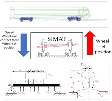
During the simulation process, the track deflection response is integrated into the vehicle model using the SIMAT co-simulation interface. The specific co-simulation principle is shown in Fig. 1. Firstly, the vehicle speed, wheel-rail contact force, and wheelset position from SIMPACK are inputted into the rail model. After calculation by the rail model, the actual vibration characteristics of the rail are outputted to the SIMPACK model. Due to changes in the rail's vibration characteristics, the wheel-rail contact relationship changes, ultimately leading to changes in the wheel-rail contact force. Then, the new wheel-rail force is inputted into the rail model again.
Fig. 1Co-simulation schematic diagram
2.2. Model validation
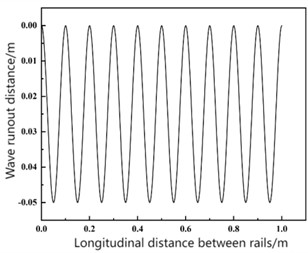
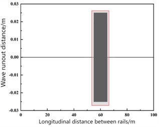
A 10-meter section of rail with corrugation was configured in the simulation, exhibiting a waveform illustrated in Fig. 2(a). The corrugation was characterized by a wavelength of 100 mm and a depth of 0.05 mm. In SIMPACK, set up a 100-meter-long straight track and apply the harmonic excitation corresponding to the aforementioned rail corrugation at the range of 55 to 65 meters. The corresponding track irregularity is shown in Fig. 2(b), where the red box indicates the added corrugation excitation, and the vertical irregularity of the remaining track is set to 0.
Fig. 2Corrugation waveform and track irregularity of the simulated rail section
a)
b)
If the axle box vibration acceleration coincides with the wave grinding frequency , then the wave grinding pass frequency satisfies the following relationship with vehicle speed and wave grinding wavelength :
Set the sampling frequency to 2000 Hz and the vehicle speed to 60 km/h. According to Eq. (1), the pass frequency corresponding to this wave-induced vibration condition is 166.7 Hz.
The vertical axle box vibration signal in the wave-grounding section is shown in Fig. 3(a). The peak values at the start and end points of the wave-grounding section are significantly higher than those in other sections. This indicates that substantial impact vibrations occur when the vehicle enters and exits the wave-grounding area, significantly affecting operational smoothness and safety. The 55-65 m section incorporates wave-induced excitation, where axle box acceleration is markedly higher than in other sections. This confirms axle box acceleration effectively reflects the time-domain characteristics of wave-induced sections.
The frequency domain information of the axle box vertical vibration signal in the wave-grinding section is shown in Fig. 3(b). The first-order vibration frequency of the axle box vertical vibration is 166.7 Hz, consistent with the wave-grinding frequency. This confirms that axle box acceleration can reflect the frequency domain characteristics of the wave-grinding section.
Fig. 3Simulation verification of shaft box vertical vibration acceleration
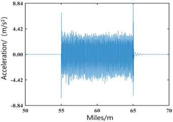
a) Vertical vibration acceleration signal in spatial domain
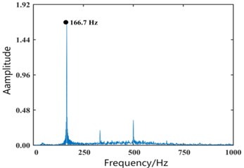
b) FFT spectrum
The frequency of axlebox acceleration matches that of wave-induced wear, indicating the high accuracy of the adopted model. This also confirms that vertical vibration acceleration of the axlebox can reflect the time-domain and frequency-domain characteristics of wave-induced wear, making it feasible to diagnose wave-induced wear using vertical vibration acceleration of the axlebox.
3. Waveform signal extraction and analysis
The EWT algorithm demonstrates excellent performance across various metrics and exhibits greater flexibility and adaptability than WPD and VMD algorithms [6-7], making it more suitable for decomposing axlebox acceleration signals.
Based on the above, this paper improves the EWT-OSTU algorithm to achieve adaptive decomposition of vertical vibration acceleration in axleboxes.
3.1. Classification standards for Hamamatsu
The rail wave wear index method, proposed by Liu Zhaojiao et al. [8], enables more effective evaluation of short-wave track irregularities and exhibits excellent repeatability. This paper employs the rail wave wear index as an evaluation metric. The index is computed from the axlebox vertical acceleration after EWT-OSTU reconstruction. First, the moving root mean square (RMS) of the reconstructed signal is calculated with a window length of 0.25 m:
where corresponds to 0.25 m of track. The track is then divided into 20 m segments, and the maximum RMS value within each segment, , is extracted. Finally, the corrugation index (in dB) for a segment is defined as:
where is the mean of the maximum RMS values over all segments. The severity levels are categorised as shown in Table 1. This index has been widely adopted in Chinese metro maintenance practice and provides a repeatable proxy for rail surface condition.
Table 1Classification of rail bobbing grades
Bobbing grades | Bobbing index / dB | Degree of bobbing | Polishing suggestions |
0 | < 5 | Non bobbing | – |
1 | 5-10 | Slight | Continuous monitoring without polishing |
2 | 10-20 | More serious | At least arrange an annual polishing plan |
3 | > 20 | Extremely serious | It should be polished in time |
3.2. Validation of the EWT-OSTU algorithm based on simulated signals
Simulating severely corrugated track conditions, the vertical acceleration amplitude of axle boxes in corrugated sections significantly exceeds that of normal sections, making them easily distinguishable. To validate the efficacy of the EWT-OSTU algorithm in extracting corrugation features, a dataset representative of mild corrugation (Grade 1) was chosen for analysis. This typical case, characterized by a wavelength of 150 mm and a depth of 0.02 mm, was sourced from the established classification results.
The time-domain plots and energy spectra of the filtered signal and decomposed sub-signals are shown in Fig. 4. After EWT decomposition, two IMF components were obtained: IMF1 contained substantial low-frequency track excitation signals, while the primary wave-grinding components were concentrated in IMF2, exhibiting relatively pure signal composition with a dominant vibration frequency matching the wave-grinding frequency.
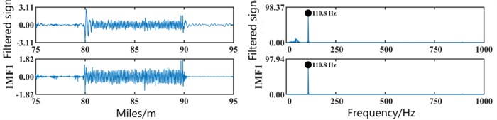
Finally, the signal with the highest energy and correlation coefficient was selected for reconstruction using the OSTU algorithm. The reconstructed signal results are shown in Fig. 5, successfully separating the wave-grinding signal from the original signal.
Fig. 4First EWT decomposition of algorithm validation data
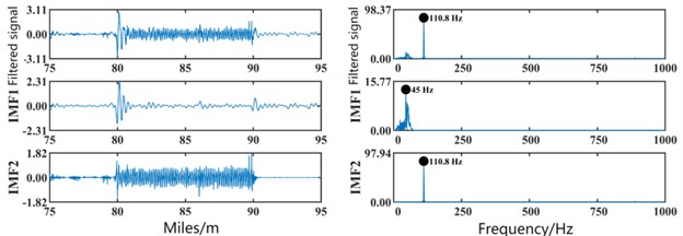
Fig. 5Algorithm validation data OSTU reconstruction result map
4. Intelligent diagnosis of rail wave wear based on actual measurement data
To further process the data obtained after completing the EWT-OSTU signal decomposition, this paper proposes a CNN–LSTM wave grinding diagnosis model and validates the model using actual line data.
4.1. CNN–LSTM fault diagnosis model
4.1.1. Components of a fault diagnosis model
Convolutional neural networks (CNNs) are a common model in deep learning [9], excelling at extracting static features. However, CNNs lack memory capabilities and cannot capture dynamic features in data. Long Short-Term Memory (LSTM) networks are a specialized type of RNN designed to address the long-term dependency issues inherent in traditional RNNs. They effectively capture and process long-term dependencies in sequences by introducing gating mechanisms.
While CNNs can extract features from axle box signals, not all statistical features are diagnostically useful. Some features not only increase computational burden but may also reduce fault classification accuracy. This paper introduces LSTMs on top of CNNs. Through their gating mechanism, LSTMs can effectively capture long-term dependencies within sequences. This capability is particularly advantageous for capturing the dynamic patterns within axlebox vibration acceleration signals. The integration of CNN and LSTM facilitates a holistic feature mining process, which thereby significantly improves the identification of wheel-rail wear characteristics from the signals.
4.1.2. Preprocessing of the actual measurement dataset
The instance dataset, denoted as , serves as the training dataset for CNN-LSTM learning, where each element is referred to as a sample. Each sample comprises two components: an -dimensional vector and an integer variable . consists of axle box vertical acceleration and vehicle velocity data collected by LANCE sensors, termed features, while is calculated from the wave-worn factor and serves as the label.
Rail wave wear exhibits temporal continuity. Based on investigations of actual wave wear failure data [10], samples are constructed using 20 m as the basic unit length. Each sample includes feature : signals reconstructed via EWT-OSTU decomposition of axle box vertical acceleration and vehicle speed data collected within 20 m; and label generated by referencing the severity grade of wave wear indices within that 20 m data segment. To ensure consistent data volume across all samples, the field-acquired axlebox vertical acceleration and speed data, which are originally sampled at a fixed frequency, undergo a conversion to equidistant spatial intervals based on a 0.02 m unit. Acceleration root mean square (RMS) values correlate closely with track condition; thus, acceleration RMS is calculated for each 0.02 m interval as an acceleration data point within the sample. Train operating speed influences the amplitude of axlebox vertical vibration acceleration data. The root mean square velocity for each 0.02 m interval serves as one operating speed factor within the sample.
In summary, a single feature comprises a set A of 1000 acceleration RMS values within a 20 m span and 1000 operating speed factors :
where, is a 1000×2 matrix.
The procedure for determining the label is outlined as follows: first, the original axle box vertical acceleration data is segmented into 20-meter sections. Each section is processed through EWT-OSTU reconstruction and decomposition. The reconstructed signals from all sections are then concatenated to form a sequence that aligns with the original signal in length.
4.1.3. Overall structure of the fault diagnosis model
We propose a CNN–LSTM model based on empirical wavelet transform, whose structure is shown in Fig. 6.
Fig. 6Structure of CNN-LSTM model based on EWT-OSTU decomposition
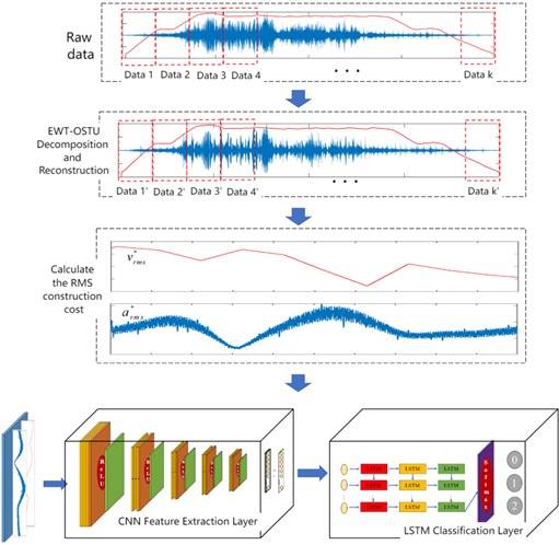
The input sequence is first processed by a CNN for spatial feature extraction. The resulting feature sequence is then fed into an LSTM to model the temporal dependencies. This approach effectively reduces the sequence length fed into the LSTM, as the CNN extracts local features from the sequence, allowing the LSTM to focus only on critical information within the sequence and improving training efficiency. Due to the presence of substantial interference noise in the raw axle box signal, training results may be compromised. Following the data preprocessing workflow outlined in the previous section, the raw signals undergo preprocessing. Subsequently, the sub-signals are calculated for their RMS values as described above and used for training the CNN.
The CNN consists of five convolutional layers, each followed by batch normalisation and a ReLU activation. The kernel sizes, strides, and output channels are detailed in Table 2. After each convolution, a max-pooling layer with size 2×1 and stride 2 reduces the spatial dimension. The final CNN output is a 64×30 feature map, which is flattened and fed into a three-layer LSTM with 64 hidden units per layer. A dropout rate of 0.5 is applied after each LSTM layer to prevent overfitting. The model is trained using the Adam optimizer with an initial learning rate of 0.001 for 100 epochs, and the cross-entropy loss is used as the objective function. Early stopping based on validation loss is employed to avoid overtraining.
Table 2Structure and parameters of the CNN–LSTM model
Layer | Number of kernels | Size / stride | Units | Input size | Output size | Activation function | Parameter |
Conv1 | 4 | 3×2/1×1 | 1×1000×2 | 4×1000 | relu | 24 | |
BN | 4×1000 | 4×1000 | 8 | ||||
Pool | 2×1/2×1 | 4×1000 | 4×500 | ||||
Conv2 | 8 | 3×1/1×1 | 8×500 | 8×500 | relu | 96 | |
BN | 8×500 | 8×500 | 8 | ||||
Pool | 2×1/2×1 | 8×500 | 8×250 | ||||
Conv3 | 16 | 3×1/1×1 | 16×250 | 16×250 | relu | 384 | |
BN | 16×250 | 16×250 | 32 | ||||
Pool | 2×1/2×1 | 16×250 | 16×125 | ||||
Conv4 | 32 | 3×1/1×1 | 32×125 | 32×125 | relu | 1536 | |
BN | 32×125 | 32×125 | 64 | ||||
Pool | 2×1/2×1 | 32×125 | 32×62 | ||||
Conv5 | 64 | 60×1/1×1 | 32×62 | 64×61 | relu | 122880 | |
BN | 64×61 | 64×61 | 128 | ||||
Pool | 2×1/2×1 | 64×61 | 64×30 | ||||
LSTM | 64 | 64×30 | 64×1 | tanh | 89600 | ||
Fully connected | 3 | 64×1 | 1×3 | 195 | |||
Classification | 3 | 1×3 | 1×3 | ||||
Total | 214963 |
The proposed CNN-LSTM intelligent diagnostic model, which utilizes EWT–OSTU for signal decomposition and reconstruction, is architecturally organized into four dedicated functional tiers: the data acquisition layer, the data preprocessing layer, the feature extraction layer, and the fault classification layer. The specific roles of each layer are detailed below:
(1) Raw Data Acquisition Layer:
This layer is responsible for collecting the raw signals of axle box vibration acceleration and vehicle velocity. The collected data is subsequently partitioned into fixed-length segments based on a 20-meter travel distance.
(2) Data Preprocessing Layer:
This layer executes the EWT-OSTU decomposition and reconstruction algorithm on the segmented raw data to generate relevant sub-signals. For each of these sub-signals, it calculates the Root Mean Square (RMS) values for both velocity and axle box vertical vibration acceleration at consistent spatial intervals of 0.02 m, thereby constructing the input samples. Given that the state of rail wave wear is strongly correlated with axlebox vertical vibration acceleration – a parameter that is itself influenced by vehicle speed – a secondary normalization procedure is applied to the acceleration RMS data. This process normalizes the acceleration data using the effective minimum and maximum speeds to derive a standardized speed factor, as defined by the following equation:
(3) CNN Feature Extraction Layer.
This layer is responsible for identifying local spatial patterns within the input samples through a convolutional neural network. The network architecture incorporates five convolutional layers utilizing the ReLU activation function for non-linear transformation. Each convolution is followed by a max-pooling operation with a kernel size of [2,2] to downsample the feature maps. The processing of raw data through this CNN architecture results in a refined feature vector that encapsulates the salient spatial information.
(4) LSTM Fault Classification Layer.
The feature vectors produced by the preceding CNN layer are flattened into a one-dimensional sequence and subsequently introduced to a three-layer LSTM network. This module is tasked with capturing the temporal dynamics and long-range dependencies inherent in the signal. The integration of CNN for spatial analysis and LSTM for temporal modeling creates a synergistic framework that markedly improves the detection of wave abrasion characteristics from the axle box vibration data.
After training through each layer, the training set achieves high accuracy, but the test set accuracy is sometimes unsatisfactory. This may indicate overfitting in the model. To address this, Dropout technology is incorporated into the LSTM layer to mitigate overfitting.
The optimization process involves multiple iterations of parameter adjustment to minimize the objective function, for which the cross-entropy loss is selected.
After EWT-OSTU decomposition, the original data eliminates substantial noise, increasing the proportion of effective information.
4.1.4. CNN-LSTM model evaluation metrics
The evaluation of model performance necessitates the employment of multiple metrics. Given that the diagnosis of rail wave abrasion is formulated as a multi-class classification task in this work, standard evaluation measures for such problems are utilized. These include accuracy, precision, recall, F1 score, the ROC curve, AUC, and the confusion matrix. A confusion matrix provides a tabular summary of the model's predictions against the true labels. Fundamental metrics like accuracy, precision, and recall are derivable from this matrix. Precision, specifically defined as the ratio of correctly identified positive instances to all instances predicted as positive by the model, is given by Eq. (6):
Recall measures the proportion of actual positive samples that the model correctly predicts as positive, as shown in Eq. (7):
The score serves as the harmonic mean of precision and recall, offering a balanced assessment of a model's predictive accuracy and its ability to capture all relevant instances, as defined by Eq. (8): score is the harmonic mean of precision and recall, comprehensively evaluating a model's accuracy and completeness, as shown in Eq. (8):
The relationships between TP, FP, FN, and TNTN in Eq. (6)-(8) are shown in Table 3.
Table 3Parameters for the calculation of multiclassification indicators
Label | 0 (Predictive Negative Class) | 1 (Predictive Positive Class) |
0 (Actual negative class) | True Positive (TP) | False Negative (FN) |
1 (Actual positive class) | False Positive (FP) | True Negative (TN) |
4.2. Line test data analysiss
The study selected multi-segment inter-platform data from the full-line dataset as the test model dataset. The dataset was divided into training and test sets. To ensure an unbiased evaluation of generalization capability, the dataset was split based on different operational runs: data from several complete inter-station segments were reserved exclusively for testing, while all remaining segments from other runs were used for training. This separation guarantees that no spatial or temporal overlap exists between the two sets, thus avoiding data leakage and providing a more realistic assessment of model performance on unseen track sections.
Fig. 7 shows the time-domain plots of axlebox vertical acceleration between platforms. In addition to the original axlebox acceleration data, the figure also displays the time-domain plots of processed axlebox acceleration data. This processed data was obtained by stitching together segments processed at 20-meter intervals using the EWT-OSTU method.
Fig. 7Time domain information map of the original data of the test set
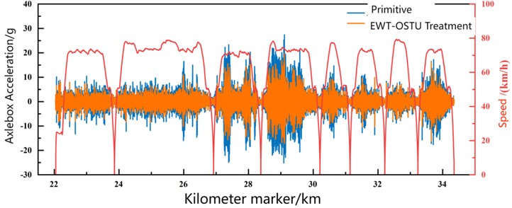
Fig. 7 demonstrates the denoising efficacy of the EWT-OSTU algorithm on the original axle box vertical vibration acceleration. The processed signal maintains most of the meaningful information from the raw data but with a substantially improved signal-to-noise ratio. This enhancement facilitates more effective identification and extraction of wave-wear features by the subsequent CNN-LSTM model.
The dataset exhibits a pronounced class imbalance, which is reflected in the composition of the training set. Out of the total 13,000 training samples, the distribution is as follows: 9,000 belong to Class 0, 3,000 to Class 1, and 1,000 to Class 2. To counteract the bias introduced by this imbalance, class weights of 0.0769, 0.2308, and 0.6923 were incorporated into the loss function during model training. For evaluation, the test set consists of 620 data units collected from 8 inter-station segments, distributed as 507 (Class 0), 85 (Class 1), and 28 (Class 2). The test set comprises 620 samples from 8 inter-station segments, with 507, 85, and 28 samples for classes 0, 1, and 2 respectively. Detailed per-class metrics are listed in Table 4. The recall for class 1 is notably lower (0.536), mainly because some impact-rich segments from class 0 were misclassified as class 1. Nevertheless, no misclassifications occurred between class 0 and class 2, indicating that the model reliably distinguishes severe corrugation from healthy track. In practice, false alarms (class 0 → class 1) are far less critical than missed detections of severe corrugation.
The corresponding confusion matrix of the diagnostic results is presented in Fig. 8, where the horizontal and vertical axes denote the true labels and the model’s predictions, respectively. The model demonstrates robust diagnostic performance, achieving recognition rates above 85 % for all categories, which confirms the practical effectiveness of the CNN-LSTM model in identifying wave-induced grinding conditions across most track sections.
Fig. 8CNN-LSTM diagnostic result confusion matrix
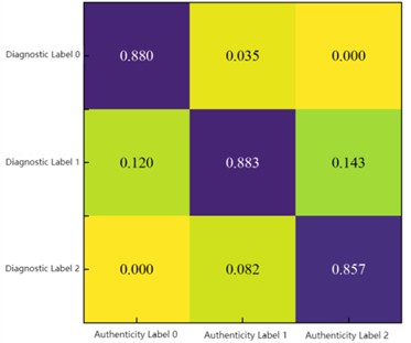
A quantitative assessment of the model’s performance on the test set is summarized in Table 4. The results confirm that the CNN-LSTM model achieves accurate identification of wave wear conditions for the majority of track segments. However, a notably lower recall rate is observed for Class 1 labels. This limitation stems mainly from the inherent class imbalance in the dataset, which led to a subset of impact-rich segments from Class 0 being erroneously assigned to Class 1. Despite this, the model attains an overall accuracy of 89.5 %, underscoring its practical utility in diagnosing wave wear under real railway operating conditions.
Table 4CNN-LSTM wave mill diagnostic result indicators
Diagnosis label | Precision | Recall | F1 Score |
0 | 0.880 | 0.993 | 0.933 |
1 | 0.883 | 0.536 | 0.667 |
2 | 0.857 | 0.774 | 0.813 |
Accuracy | 0.895 | – | – |
To more intuitively demonstrate the diagnostic effectiveness of the test set, the diagnostic results were visualized as a spatial domain image, as shown in Fig. 9. The figure reveals that most units were accurately identified, yet some units were misdiagnosed. Among the misdiagnosed data, the majority classified Class 0 samples – units without wave wear – as Class 1 samples, indicating units with minor wave wear. This may occur because localized abnormal impacts between wheelsets and rails are mistakenly identified as wave wear characteristics. Although misclassifications exist, the vast majority of errors involve overestimating the severity of wave wear. Furthermore, there is no overlap between the identified non-wave-worn units and those recommended for grinding due to severe wave wear. Therefore, applying the CNN-LSTM model for wave wear diagnosis and early warning on actual rail lines is feasible.
To provide a preliminary assessment of robustness against speed variations, the test set includes inter-station segments covering a speed range from 40 to 80 km/h. The model maintained high accuracy across this range, with no systematic degradation observed at either low or high speeds. While a more comprehensive evaluation – e.g., training on one speed range and testing on another – would further quantify robustness, the current test set already reflects realistic operational diversity. Future work will include dedicated cross-speed experiments to validate the model’s speed invariance.
Fig. 9Diagnostic results of CNN-LSTM model test set
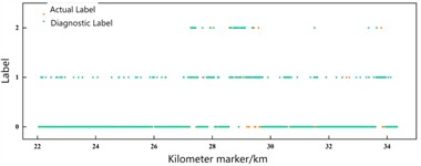
a) Diagnostic results for all units
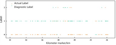
b) Error recognition unit
4.3. Model visualization
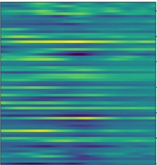
Generally speaking, deep learning models are black-box models, making it difficult to understand their internal mechanisms. This paper visualizes the hidden layer signals of the CNN-LSTM model to explore the underlying inference process. Fig. 10 displays the activation status of each hidden layer, where yellow indicates activated units and green indicates deactivated units. It is challenging to distinguish fault types from the first convolutional layer, but as the network deepens, the feature maps become increasingly clear. After the feature vectors extracted by the CNN layer undergo further processing in the LSTM layer, the features become more pronounced, facilitating wave grinding recognition.
Fig. 10CNN-LSTM hidden layer signal visualization
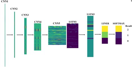
Fig. 11CNN extracted data feature map
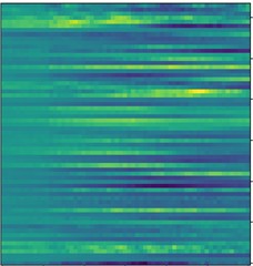
a) Non bobbing
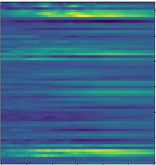
b) Slight
c) More serious
The fifth-layer convolutional outputs for different data categories were then examined. Inputs with and without wave-grinding signals were converted from 1000×2 input signals into 64×61 matrices according to Table 3. Fig. 11 indicates that different signal types generated distinct feature matrices. The yellow regions in the feature maps extracted by wave-grinding CNNs varied across categories, with corresponding activation neurons also differing. This demonstrates that CNN feature extraction occurs automatically without manual intervention.
Before inputting into LSTM training, the convolutional output vector from the fifth layer undergoes regularization processing, feature extraction via pooling layers, and dimensionality reduction. The resulting feature vector is shown in Fig. 12.
After undergoing the aforementioned processing, the 64×61 matrix transforms into a matrix with more distinct features, facilitating LSTM extraction of signal characteristics and enhancing the accuracy of wave-grinding classification diagnosis.
Fig. 12LSTM input feature vector map

a) Non bobbing

b) Slight

c) More serious
5. Conclusions
1) Through a simplified model of the wheel-rail system, combined with theoretical and simulation verification, it was demonstrated that detecting rail wave wear via axle box vertical vibration acceleration is feasible. Sub-signals decomposed by EWT were examined using the OSTU algorithm. Subsequently, simulation data were classified based on wave wear indices. A segment of simulation data was selected to validate the EWT-OSTU algorithm, demonstrating its capability to extract wave wear components from axlebox vertical vibration acceleration.
2) Based on EWT-OSTU signal decomposition, a CNN-LSTM wave wear diagnostic model was proposed. Using multi-section platform data from an actual line as the test set, the model achieved an 89.5 % validation accuracy, demonstrating the feasibility of applying the CNN-LSTM model for wave wear diagnosis and early warning on operational lines.
3) It should be noted that the current study does not explicitly account for variations in vehicle type, wheel wear state, suspension conditions, or environmental factors such as temperature and humidity. These factors can influence the axlebox vibration signature and may affect the model’s generalisation performance. Future work could explore domain adaptation or adversarial training techniques to improve robustness across different operational conditions.
References
-
H. Y. Zhu et al., “Progress in the study of rail corrugation,” (in Chinese), Journal of Traffic and Transportation Engineering, Vol. 21, No. 3, pp. 110–133, 2021, https://doi.org/10.19818/j.cnki.1671-1637.2021.03.006
-
G. Shen, X. H. Zhang, and M. H. Guo, “Measurement and analysis of wavy wear on curved rails in metro,” (in Chinese), Urban Mass Transit, Vol. 14, No. 4, pp. 53–54, 2011.
-
S. M. M. Gazafrudi, D. Younesian, and M. Torabi, “A high accuracy and high speed imaging and measurement system for rail corrugation inspection,” IEEE Transactions on Industrial Electronics, Vol. 68, No. 9, pp. 8894–8903, Aug. 2020, https://doi.org/10.1109/tie.2020.3013748
-
D. Wei, X. Wei, Y. Liu, L. Jia, and W. Zhang, “The identification and assessment of rail corrugation based on computer vision,” Applied Sciences, Vol. 9, No. 18, p. 3913, Sep. 2019, https://doi.org/10.3390/app9183913
-
N. Rezazadeh, M. de Oliveira, D. Perfetto, A. de Luca, and F. Caputo, “Classification of unbalanced and bowed rotors under uncertainty using wavelet time scattering, LSTM, and SVM,” Applied Sciences, Vol. 13, No. 12, p. 6861, Jun. 2023, https://doi.org/10.3390/app13126861
-
R. R. Coifman, Y. Meyer, and M. V. Wickerhauser, “Wavelet analysis and signal processing,” in Wavelets and their applications, New York, NY: Jones and Bartlett, 1992, pp. 153–178, https://doi.org/10.1007/978-1-4684-6393-4_5
-
K. Dragomiretskiy and D. Zosso, “Variational mode decomposition,” IEEE Transactions on Signal Processing, Vol. 62, No. 3, pp. 531–544, Jan. 2014, https://doi.org/10.1109/tsp.2013.2288675
-
J. Z. Liu et al., “Track impact index method for assessing short-wave unevenness disease of high-speed railway tracks,” (in Chinese), China Railway Science, Vol. 37, No. 4, pp. 34–41, 2016, https://doi.org/10.3969/j.issn.1001-4632.2016.04.06
-
H. Dou et al., “A review on the interpretability of convolutional neural networks,” (in Chinese), Journal of Software, Vol. 35, No. 1, pp. 159–184, 2024, https://doi.org/10.13328/j.cnki.jos.006758
-
Z. Wang, R. Liu, F. Wang, and Y. Tang, “Development of metro track geometry fault diagnosis convolutional neural network model based on car-body vibration data,” Proceedings of the Institution of Mechanical Engineers, Part F: Journal of Rail and Rapid Transit, Vol. 236, No. 9, pp. 1135–1144, Mar. 2022, https://doi.org/10.1177/09544097221080366
About this article

This work was supported by the National Natural Science Foundation of China under Grant 52272406.
The datasets generated during and/or analyzed during the current study are available from the corresponding author on reasonable request.
Yanqing Gong: supervision, resources, writing-review and editing. Cheng Zhu: software, validation, writing-review and editing. Jiankun Xie: methodology, formal analysis, writing-review and editing. Tingzhou Hu: data curation, visualization, writing-review and editing, corresponding author. Jie Hu: conceptualization, supervision, project administration, formal analysis, data curation, writing-review and editing. All authors have read and agreed to the published version of the manuscript.
The authors declare that they have no conflict of interest.

