Abstract
An integrated robotic system, comprising an industrial serial manipulator and a custom bending head, is proposed to address the limitations of traditional CNC pipe bending machines, such as frequent physical interference and challenges in single-step forming for intricate pipe fittings. The system is designed to ensure high processing efficiency and accurate shaping for complex tubular components. In this research, the coordinate system fixed to the linkage is established using the Denavit-Hartenberg (D-H) convention to represent the bending motion. The inverse kinematics for a given end-effector pose is resolved via a sequential analytical algorithm utilizing joint angle parameterization. A simulation model is developed using MATLAB’s Multibody toolbox to validate the proposed inverse kinematics method. The accuracy of the solution is verified through a rigorous comparison between simulation results and experimental pose data, demonstrating the system's viability and precision for automated pipe bending scenarios.
1. Introduction
Pipe bending is the plastic-forming process of metal tubes into specified radii, bend angles, and 3D shapes. The growing demands for innovation and functional integration have significantly elevated the importance of high-performance bent components in tube forming technology. As a critical process in metal pipe plastic processing [1], pipe bending is extensively employed to manufacture parts for aerospace, petrochemical, automotive manufacturing, and other fields [2], [3]. With the ongoing technological upgrading and industrial transformation within these sectors [4], [5], there is an increasing need for components possessing complex features [6], [7], such as highly intricate spatial axes, small bending radii, and multiple curvatures. Consequently, to meet the precision and performance requirements of these high-standard bending parts, it is imperative to adopt intelligent pipe bending equipment [8] that offers high flexibility and an advanced level of automation.
Currently, the predominant equipment for pipe bending is the computer numerical control (CNC) pipe bending machine, which operates a bending head via a computerized system. However, this equipment typically relies on manual loading and unloading, resulting in high labor costs. Furthermore, its substantial footprint increases factory space expenses. More critically, when processing pipe fittings with high complexity, such machines exhibit insufficient flexibility and are prone to interference with the already bent sections, often preventing single-step completion [9]. Despite advancements in robotic manufacturing, a critical research gap remains in achieving highly efficient, single-step forming for complex spatial pipe fittings without physical interference. Existing robotic bending solutions heavily rely on computationally expensive numerical kinematics. To address this gap, a novel robotic pipe bending system is proposed. This system integrates the high efficiency, flexibility, and precision of an industrial serial robotic manipulator with the forming function of a bending head to achieve continuous pipe bending. In contrast to traditional CNC machines, the robotic system offers greater operational flexibility, faster response times, a reduced footprint, and integrated automated loading and unloading capabilities, resulting in a higher degree of automation. This robotic bending technology can fulfill the demand for the rapid forming of complex pipe fittings and is poised to advance the development of digital pipe bending and forming processes.
The effective integration of a pipe bending actuator with an industrial serial robot arm for pipe bending applications requires careful consideration of their compatibility and adaptability. To achieve optimal synergy and enhance overall processing efficiency and quality, it is imperative to refine the bending actuator to match the robot’s operational characteristics or to develop novel control strategies for their collaboration. This approach is essential to ensure processing stability, guarantee forming accuracy, and fully utilize the robotic arm’s inherent flexibility.
At present, domestic and foreign robot research and development and manufacturing enterprises have some preliminary design schemes. For the improvement of the pipe bending processing actuator, the domestic Wu Jianbo, Li Guanhong [10] and other disclosed a metal processing pipe bending device, the device simplifies the traditional pipe bending head, only composed of the pipe body and mounting plate, small size, light weight, high flexibility, making it very suitable for use in combination with industrial series robot arm. Li Cong, Huang W. [11]anyong, a researcher of Fanalke Robot Company, etc., disclosed a full-servo robot bending machine device, which uses a full-servo motor to control the driving mechanism of the bending machine actuator, improving the accuracy of bending machine processing, and designed the connection mode of the bending machine actuator and the industrial series robot arm, which is highly integrated with the industrial series robot arm and the bending machine head.
For the cooperation between the pipe bending actuator and the robot, the mainstream method can be divided into two kinds. integrated and collaborative. Among them, the pipe bending processing actuator of the cooperative cooperation mode is separated from the industrial series robot arm and works together as an independent device. In this design, the industrial series manipulator is responsible for material handling and positioning, while the pipe bending manipulator focuses on the bending task. For example, the research team of Fanuc Company in Japan, including Ni Ye, Li Kunju [12] and other researchers, developed a robot pipe bending workstation, which is a typical example of the cooperation between industrial series robot arm and pipe bending actuator. Compared with the cooperative mode, the integrated mode directly inserts or integrates the pipe bending processing actuator into the output shaft of the end joint of the industrial series manipulator, making the two become a closely integrated unit. In this configuration, the robot itself is responsible for the operation of the bending process, using its flexibility and high-precision control to perform the bending task.
The tubular bending robot includes a six-axis robot and an end-effector. Robot kinematics, particularly the inverse kinematics solution, is crucial for trajectory planning and remains a key area of research. Currently, both domestic and international studies on solving the inverse kinematics of six-axis robots are well-established, utilizing methods such as analytical, numerical, and geometric approaches [13]. However, the bending robot is installed at the end of the bending head, can not fully apply the traditional robot inverse kinematics solving method, so it is necessary to carry out targeted research to solve the problem of its inverse kinematics solving, to ensure the processing accuracy, stability, flexibility, safety and adaptability of the bending robot in the execution of processing tasks. Compared to widely used numerical methods (e.g., Jacobian-based iterative solvers or optimization-driven approaches) which suffer from high computational overhead and non-convergence near singularities, the novelty of this paper lies in a targeted joint angle parameterization approach derived from the system's unique mechanical coupling. Because the 7th joint is mechanically driven by the 6th joint via a proportional transmission, they can be treated as a single unit during decoupling. By customizing these coupled angles for attitude control, the remaining joints can be solved via a deterministic, closed-form analytical algorithm. This deeply integrated mechanical-kinematic approach inherently avoids algorithmic dead-locks and meets the strict real-time control requirements of industrial pipe bending.
2. Kinematic modeling of pipe bending robot
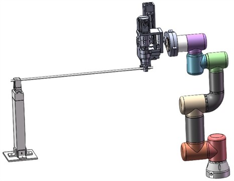
The structure of the tubular bending robot is shown in Fig. 1. The main body of the robot is a six-degree of freedom series manipulator, each joint is a rotating joint, and the bending head is installed at the end. It is composed of a pipe bending spindle, a clamping mechanism, a guiding mechanism and a rotator. This configuration has the characteristics of good flexibility, large working range, and multi-directional and multi-degree of freedom movement, which is very suitable for complex machining tasks. It should be emphasized that the significant torque required for the plastic deformation of the metal pipe is entirely generated by the dedicated servo-driven bending spindle within the head. The 6-axis industrial manipulator, selected for its high-payload capacity and structural rigidity, primarily serves to dynamically position the head and safely withstand the static reaction forces during the bending process without overloading its joint motors.
Fig. 1Structure diagram of pipe bending robot
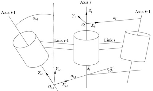
The kinematic modeling of the pipe-bending robot uses the improved Denavit-Hartenberg (D-H) method [14]. This method involves creating a coordinate system at each robot joint and deriving the kinematic model through homogeneous transformations. The improved D-H method modifies the fixed coordinate system of the connecting rod, expanding its applicability.
In the modified D-H approach, the robotic manipulator consists of joint axes and connecting links. Four parameters (, , , ) define the relationship between the axes and links, as illustrated in Fig. 2, with their definitions provided below.
(1) represents the length of the connecting rod, specifically the distance along the common vertical line between the axes of joints and .
(2) is the rotational angle of the connecting rod, defined as the angle between the axes of joints and projected onto a plane perpendicular to the common vertical line between them.
(3) denotes the displacement of the connecting rod, measured along the common axis between two adjacent rods. It corresponds to the distance between the vertical lines of the and axes, projected onto the axis of joint .
(4) is the rotational angle of the joint, describing the angle between two adjacent rods as they rotate around their shared axis.
To represent the relationship between the robot’s motion and the connecting rods, a coordinate system must be established at each joint. The system’s origin and axis directions follow these guidelines.
The origin of the coordinate system. The origin of the coordinate system is the foot of the common vertical line between the joint axis and the joint i axis on the axis of the joint axis.
Fig. 2Schematic diagram of the improved D-H method
The origin is located at the base of the common vertical line between the axes of joints and , placed on the axis.
axis: the direction is the direction of the common vertical line between the joint axis and the joint axis.
axis: Perpendicular to the axis and axis the direction follows the right hand rule.
Based on these principles, the pipe bending robot in this study is modeled. To illustrate this, the robot’s initial configuration is shown in Fig. 3. The head part primarily performs rotation and displacement around the pipe fitting, and the seventh axis moves proportionally with the sixth axis. Thus, the connecting rod is considered equivalent to the seventh axis. The coordinate system illustration is presented in Fig. 4.
Fig. 3Robot’s initial configuration
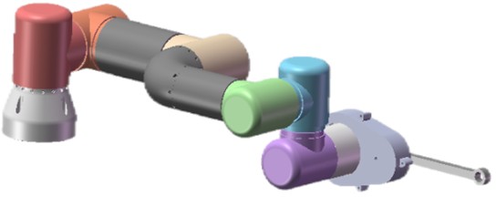
Fig. 4Schematic diagram of robot D-H modeling
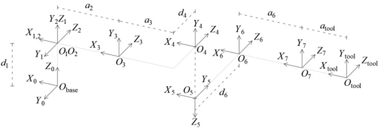
Based on the actual dimensions of the pipe bending robot, the corresponding D-H parameters are determined, with the details provided in Table 1. Notably, the initial angles of the 2nd joint and the 4th joint are both set to 90°. It is important to highlight that the 7th joint is powered by the 6th joint. The power from the 6th joint is transmitted to the 7th joint through the gear mechanism in the rotator. As a result, a gear transmission ratio 1.15 exists between the rotation angles of the sixth and seventh joints, as described below:
Table 1Improved D-H parameters of pipe bending robot
Joint number | / (°) | / (mm) | / mm | / (°) |
1 | 0 | 0 | 144 | 0 |
2 | 90 | 0 | 0 | –90 |
3 | 0 | –264 | 0 | 0 |
4 | 0 | –236 | 106 | –90 |
5 | 90 | 0 | 114 | 0 |
6 | -90 | 0 | 67 | 0 |
7 | 0 | –82.5 | 0 | 0 |
Tool | 0 | –200 | 0 | 0 |
3. Solving the kinematics of the bending robot
3.1. Forward kinematics solution of pipe bending robot
Forward kinematics involves determining the pose [15], [16] of the robot’s end-effector by knowing the joint angles. Once the kinematic model is established, it must be linked with the coordinate systems. The transformation between adjacent coordinate systems is typically achieved through translation and rotation. The tubular bending robot is a series connection of the end tool shaft and a standard six-axis robot arm, with a proportional transmission relationship between the sixth axis and the end tool shaft. Thus, the forward kinematics solution for the tubular bending robot can be treated as that of a six-axis robot arm, with the homogeneous transformation matrix of the end tool shaft connected in series. The steps and sequence for this process, as outlined by the improved D-H parameter method, are as follows.
(1) The angle of rotation of the axis around the axis, so that the axis is parallel to the axis.
(2) The origin of the coordinate system is translated a distance along the axis, so that the axis is collinear with the axis.
(3) The axis is rotated about the axis through an angle , such that the axis becomes parallel to the axis.
(4) The origin of coordinate system is translated along the axis by a distance , such that coordinate system completely coincides with coordinate system . Therefore, the transformation matrix between coordinate systems and is given by:
By bringing the parameters in Table 1 into Eq. (2), the transformation matrix between the joints of the robot can be calculated as:
The total transformation matrix of the forward kinematics of the bending robot is the Eq. (11):
3.2. Solving the inverse kinematics of the pipe bending robot
The inverse kinematics is the basis of robot control. Different from the forward kinematics of robots, the inverse kinematics solution is to solve the angle [17], [18] of each joint when the position and pose of the end effector of the robot are known. Inverse kinematics solutions typically involve analytical, numerical, and geometric approaches. The bending robot in this paper has seven joint axes, and its configuration does not meet the Pieper principle. If the inverse solution is directly solved for the whole, only numerical method can be adopted, which is of great computational complexity, long time and high requirements on the initial value of iteration, and is not suitable for real-time control requirements [19], [20]. A solution method using joint angle parameterization is proposed in this paper to address the robot's inverse kinematics. This novel parameterization strategy effectively reduces the system's dimensionality, transforming a complex multi-axis configuration into an analytically solvable model, providing a computationally efficient alternative to conventional iterative numerical solvers.
The 7th joint of the bending robot is driven by the 6th joint, with its output angle amplified by the rotator. This results in a proportional relationship between their angles, allowing them to be treated as a single unit during decoupling calculations. To enable flexible processing, the angles of the sixth and seventh joints are customized for attitude control. The angles of the remaining joints are computed analytically to solve the robot's inverse kinematics.
Among them, the sixth joint and the seventh joint are the custom angle, and the expression of its transformation matrix can be obtained as follows, with (abbreviation of ), (abbreviation of ), is the gear ratio coefficient:
The end-tool matrix can be obtained according to the D-H parameter, and its expression is:
Apply the inverse matrix transformation to the Eq. (11), you can get:
Eq. (15) is the total homogeneous transformation matrix of the first to the fifth joint. The solution of this matrix should first solve the angle of the first joint, and also use the inverse matrix transformation to rewrite Eq. (15) into the following form:
Of which:
Let the (2, 4) element in the matrix product result of Eq. (16) correspond to the (2, 4) element in Eq. (17), we can get:
The solution Eq. (18) can be solved through the trigonometric identity transformation formula to get:
At this time, the that has been solved has two sets of solutions, and then solve , so that (2, 1) and (2, 2) in Eq. (16) and Eq. (17) are equal, we can get:
In combination with the above Eq. (20) and Eq. (21), it can be solved:
Corresponding to different , with corresponding solutions. Put the calculated into the corresponding homogeneous transformation matrix, and rewrite the Eq. (16) as follows by the inverse matrix transformation:
In Eq. (23), the sine function represents the sum of angles of joints 2, 3 and 4. The cosine function representing the sum of angles of joints 2, 3, and 4. While and representing the and axis positions in the operating space:
This is obtained by adding the above Eq. (26) to the Eq. (27) simultaneously squared:
By utilizing the sum-angle formulas of sine and cosine functions, and can be determined. Subsequently, is calculated using the two-variable arctangent formula:
has two values (positive and negative), there exist two solutions for . Once the values of are determined, Eq. (26) and Eq. (27) can be reformulated into the following forms:
In Eq. (30) and Eq. (31), the specific expressions of and are as follows:
Through variable substitution, the expression of can be obtained as follows:
Finally, given and , can be determined using the following equation:
Thus, with , , , and calculated and combined with the user-defined parameters and , the inverse kinematics solution for the pipe-bending robot is completed.
3.3. Singularity avoidance strategy
Furthermore, it is crucial to address the kinematic singularities commonly encountered by 6-DOF and 7-DOF robots. The analytical inverse kinematics approach proposed above inherently yields multiple solution branches. During practical trajectory planning, the controller monitors the Jacobian matrix and utilizes these multiple analytical solutions to actively switch the manipulator’s configuration, thereby effectively avoiding kinematic singularities and dead zones within the robot’s workspace.
4. Experiment and analysis of pipe bending robot
4.1. Pipe bending robot simulation model construction
The construction of the simulation model of the pipe bending robot adopts MATLAB Multibody of MATLAB Link plug-in, which exports the 3D model of Solidworks, Inventor, Creo and other modeling software into step and xml format files that can be read by MATLAB, and effectively integrates the 3D model into MATLAB for simulation and analysis [21], [22]. In the early Solidworks to create the robot model, it must be ensured that the constraints between each joint are configured for the correct coincidence and coaxial relationship, and the initial state of the assembly should meet the state requirements of the D-H parameter, so that each joint axis [23], [24] can be accurately identified when exported. The rotating head of the bending robot consists of numerous complex components, which require significant computational resources for simulation model construction. To enhance simulation efficiency, components like the bending spindle, clamping mechanism, and guide mechanism are simplified and replaced with a connecting rod model.
After building the simulation model of the robot, the next key step is to build the motor model to drive the movement of the robot joints. This paper uses the stepper motor model in Simulink, which can be quickly created by inputting the “elec_motor_stepper” command in the MATLAB command window. The motor model provides two control modes, one is position control, the other is speed control. Since the input signal received by the robot model built in the above section is angle input, the position control mode should be selected for the motor model to meet the requirements of the robot joint input.
In the input end of the motor model, in order to directly import the results of solving the inverse kinematics of the robot and the trajectory planning, the default step signal input needs to be modified to the self-defined system input signal Input1. Considering that the entire step distance of the stepper motor used is 1.8°, it is necessary to divide the angle value of the solution result by the step distance of the motor, so as to obtain the number of steps used to drive the motor, and then input the data into the motor controller in order to achieve accurate control of the robot joint [25].
At the output end of the motor model, an adder is designed to add the compensation value of the initial angle of the robot joint, so that the initial attitude of the robot can be customized. Considering that the output of the motor model is in the unit of angle, and the robot joint needs the input in radian, so the necessary conversion components are added between the two. Finally, with the help of Simulink-PS conversion element, the Simulink input signal is converted into the physical signal output, and the MATLAB simulation model is built, as shown in Fig. 5.
Fig. 5MATLAB model diagram of the bending robot
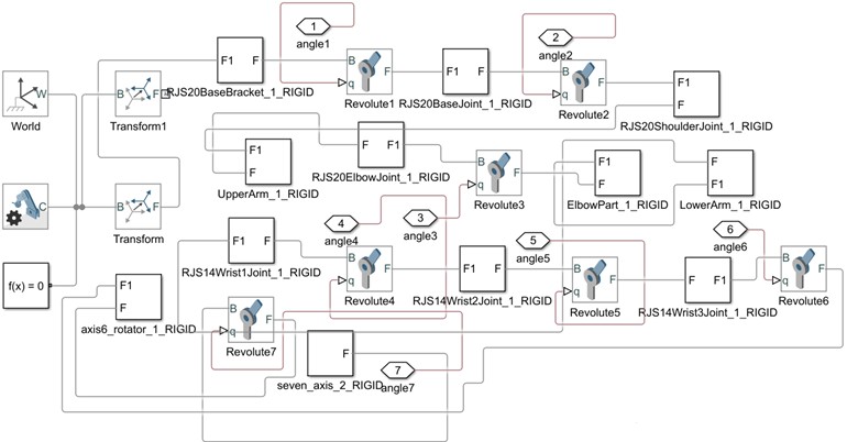
Based on the above MATLAB simulation model and motor drive model, the model can be used to verify the proposed inverse kinematics solution method based on joint angle parameterization. Specifically, the known end-pose parameters of the robot, including position and attitude , need to be given, and converted into a one-dimensional array and input to the MATLAB Function module. The code of inverse kinematics solving algorithm has been written inside the module, which is used to calculate the corresponding joint angle. These angles are then output to a motor driven model that is then passed on to the robot. Furthermore, to validate the robustness of the proposed method under complex spatial conditions, extensive simulation tests involving continuous multi-bend trajectories were conducted. The results demonstrated that the analytical solver consistently maintained high positional accuracy and real-time computational efficiency throughout the complex bending sequences.
4.2. Pipe bending robot experiment platform construction
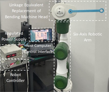
The experimental platform model includes multiple modules, as illustrated in Fig. 6.
(1) Instruction receiving module: This module contains two key sub-modules, namely, data receiving module and data verification module.
(2) Motion control module: In the motion control module, three different control strategies are implemented to adapt to different operational needs. They are point to point (PTP) control mode, joint space trajectory planning (PVT) mode and Cartesian space trajectory planning (PT) mode.
(3) Joint position module: This module realizes the data storage function, which is mainly used to store the joint angle data processed by the motion control module, so as to facilitate the robot model to read it.
(4) Data broadcast module: The data broadcast module provides a communication mechanism for the robot to distribute or share information among multiple systems, modules or devices.
The operation procedure for the experimental platform is conducted through a systematic workflow. The experimental platform model is opened in MATLAB, and the appropriate control mode is selected within the motion control module. For this study, the Cartesian space trajectory planning (PT) mode is adopted as the operating example.
Using the written MATLAB script, the joint angle sequence is computed through inverse kinematics for each interpolation point of the Cartesian space trajectory. The simulation is executed to verify that all robot joints can move continuously without encountering crashes or locking issues. Upon successful simulation, the computed joint angle values are stored in the joint position module of the experimental platform model.
During compilation and download of the platform model, the corresponding joint angle data are automatically extracted from the script workspace and transmitted to the robot motors for execution. The hardware components are then connected in sequence. Power is supplied to the voltage regulator, with the voltage adjusted to 48V (48.0 V~48.6 V). Subsequently, the robot controller is activated to supply power to the robot. The compile button at the top of the model interface is clicked to download the model and data to the manipulator controller. The successful program installation is verified through the View Diagnostic Viewer.
The control system software is executed following the operational sequence: Start → Reach initial attitude → Start trajectory movement → Return to zero → Stop. This systematic approach ensures proper initialization, execution, and termination of the robotic bending operations.
Fig. 6Experimental platform of bending robot. Photo by the second author in the laboratory of the School of Engineering, Huzhou Normal University in March 2025
4.3. Kinematic experiment and analysis of pipe bending robot
Based on the simulation model and experimental platform of the pipe bending robot established above, the kinematic experiment analysis is carried out. Specifically, it is necessary to give the known robot end pose parameters including position and attitude , and convert them into a one-dimensional array and input them into MATLAB Function module. The code of inverse kinematics solving algorithm has been written inside the module, which is used to calculate the corresponding joint angle. The experiment is mainly to verify the accuracy of the proposed inverse kinematics method for solving the bending robot.
Taking a single pose point as an example, firstly, given the end-effector pose of the bending robot as (452 mm, –173 mm, 482 mm, 60°, 0°, 90°), and the initial angle of the sixth joint as –23.64°, the angles of all joints of the robot are calculated as (0°, –31.24°, –27.32°, –36.46°, 0°, –23.64°) using the inverse kinematics solution method described above. Then, verify the accuracy of the calculated results, input these joint angles into the simulation model, and observe whether the pose of the bending robot is reasonable after the completion of movement.
Finally, the given pose is tested on the real machine of the pipe bending robot, and the actual angles of each joint of the robot can be obtained as (0.01°, –31.14°, –27.52°, –36.37°, 0°, –23.73°), and the actual pose of the end of the robot is (451.68 mm, –172.86 mm, 483.56 mm, 60.26°, 0°, 89.82°), as shown in Table 2 and Table 3. The operation results are shown in Fig. 7. Fig. 7 respectively represent the initial pose, intermediate pose and end pose of the bending robot in the actual experiment.
Table 2Comparison of theoretical pose and actual pose of the end of the pipe bending robot
(mm) | (mm) | (mm) | (°) | (°) | (°) | |
Theoretical value | 452 | –173 | 482 | 60 | 0 | 90 |
Actual value | 451.68 | –172.86 | 483.56 | 60.26 | 0 | 89.82 |
Table 3Comparison between theoretical joint angle and actual joint angle of bending robot
First axis (°) | Second axis (°) | Third axis (°) | Fourth axis (°) | Fifth axis (°) | Sixth axis (°) | |
Theoretical value | 0 | –31.24 | –27.32 | –36.46 | 0 | –23.64 |
Actual value | 0.01 | –31.14 | –27.52 | –36.37 | 0 | –23.73 |
Fig. 7Real motion pose of pipe bending robot
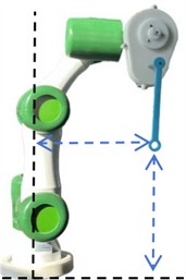
a) Starting pose
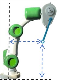
b) Motion process pose 1
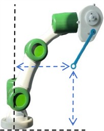
c) Motion process pose 2
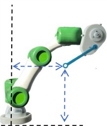
d) End pose
In the accurate test of the pipe bending robot, a specific point is chosen as the origin for pipe fitting processing, and various spatial positions are tested. Five sets of end poses are used to gather comparison data for the theoretical, simulation, and actual values of the robot's end pose, as shown in Table 4.
Table 4Comparison of theoretical, simulated, and actual values of the end effector posture of the pipe bending robot
(mm) | (mm) | (mm) | (°) | (°) | (°) | ||
The first group | Theoretical value | 364.00 | –318.00 | 482.00 | 60.00 | –20.00 | 90.00 |
Simulation value | 364.03 | –318.00 | 482.01 | 60.01 | –20.02 | 89.99 | |
Actual value | 364.17 | –318.19 | 482.10 | 60.17 | –20.14 | 89.91 | |
The second group | Theoretical value | 415.00 | 23.00 | 482.00 | 60.00 | –27.00 | 90.00 |
Simulation value | 415.02 | 23.01 | 482.00 | 60.03 | –27.01 | 90.01 | |
Actual value | 415.19 | 23.05 | 482.07 | 60.08 | –27.13 | 89.90 | |
The third group | Theoretical value | 452.00 | –173.00 | 482.00 | 60.00 | 0 | 90.00 |
Simulation value | 452.02 | –173.00 | 482.01 | 60.00 | 0 | 89.99 | |
Actual value | 451.78 | –172.87 | 482.09 | 60.16 | 0.23 | 89.82 | |
Fourth directorate | Theoretical value | 474.00 | 92.00 | 482.00 | 70.00 | 10.00 | 90.00 |
Simulation value | 474.02 | 92.01 | 482.00 | 70.01 | 9.99 | 89.99 | |
Actual value | 474.27 | 92.08 | 482.11 | 70.12 | 9.93 | 89.76 | |
Fifth directorate | Theoretical value | 517.00 | –15.00 | 482.00 | 75.00 | 17.00 | 90.00 |
Simulation value | 516.98 | –15.01 | 481.99 | 74.99 | 17.01 | 90.00 | |
Actual value | 517.29 | –15.04 | 482.04 | 75.21 | 17.18 | 90.15 | |
The kinematics error of the pipe bending robot’s end pose was analyzed by testing different processing positions to assess the accuracy of the kinematics solution. The maximum error between the theoretical and actual values is 0.29 mm, and the minimum is 0.05 mm. It is worth noting that this maximum error of 0.29 mm is partially attributed to the inherent mechanical backlash within the gear transmission system connecting the sixth and seventh joints. Although precision gears were utilized, micro-clearances during direction reversals slightly affect the absolute positioning accuracy of the end-effector.
Fig. 8Comparison data of error values of the theory, simulation and actual values of the pose of the bending robot
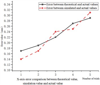
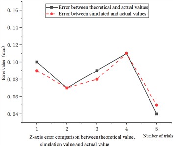
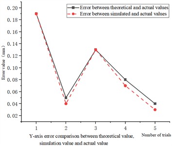
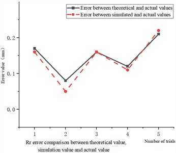
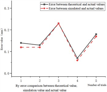
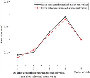
For simulation versus actual values, the maximum error is 0.31 mm and the minimum is 0.04 mm. The maximum rotation angle error between theory and actual values is 0.24°, and the minimum is 0.07°. Between simulation and actual values, the maximum error is 0.23° and the minimum is 0.065°. These results show that the motion error of the robot increases with the movement distance, but all errors remain within acceptable limits, satisfying the robot's accuracy requirements. The comparison of theoretical coordinates, rotation angles, and errors between simulation and actual values are presented in Fig. 8.
5. Conclusions
Aiming at the limitation of traditional bending machines in automation level and flexibility, an intelligent bending robot processing equipment is designed. Aiming at the mechanical structure design of the pipe bending robot, the integrated design scheme of six degrees of freedom joint manipulator and rotating head is adopted. The improved D-H method is used to model the bending robot, and the forward kinematics equation is derived. According to the configuration of the robot, a partial solution method of joint angle parameterization is proposed. By parameterizing the sixth joint angle and the seventh joint angle of the robot, the total transformation matrix is decoupled, and then the remaining joint angle is solved analytically to solve the inverse kinematics of the bending robot. The accuracy of the inverse kinematics method proposed in this paper is verified by the test of the actual experiment platform. It provides some theoretical support and practical value for the application of industrial robot in the field of bending pipe processing. Furthermore, it is important to acknowledge the inherent limitations of the proposed method. While highly efficient for specific configurations, this closed-form analytical solution lacks direct scalability to highly redundant manipulators (e.g., manipulators with more than 7 DOFs) without introducing additional constraint parameters. Additionally, the robot's reachable workspace remains bounded by mechanical joint limits, and the current model does not incorporate dynamic force feedback for tube springback compensation. These aspects will be the focus of our future research. However, it should be noted that the physical experiments in this current study were primarily conducted under no-load conditions to strictly verify the kinematic and angular accuracy of the algorithm. Conducting fully loaded physical experiments involving complex, continuous multi-bend trajectories will be the primary focus of our future work to further evaluate the system’s dynamic forming performance under real-world material resistance.
References
-
T. Wang, Plastic Processing Technology of Pipe. (in Chinese), China Machine Press, 1998.
-
J. Wu et al., “Research review and prospect of pipe bending machine,” (in Chinese), Internal Combustion Engine and Accessories, Vol. 2023, No. 8, pp. 106–108, 2023, https://doi.org/10.19475/j.cnki.issn1674-957x.2023.08.025
-
L. Zhang et al., “Design and control of three-dimensional mouldless pipe bending robot,” (in Chinese), Modern Manufacturing Engineering, Vol. 2022, No. 2, pp. 59–63, 2022, https://doi.org/10.16731/j.cnki.1671-3133.2022.02.009
-
M. Alebooyeh and R. J. Urbanic, “Neural network model for identifying workspace, forward and inverse kinematics of the 7-DOF YuMi 14000 ABB collaborative robot,” IFAC-PapersOnLine, Vol. 52, No. 10, pp. 176–181, 2019, https://doi.org/10.1016/j.ifacol.2019.10.019
-
H. Yang, H. Li, Z. Zhang, M. Zhan, J. Liu, and G. Li, “Advances and trends on tube bending forming technologies,” Chinese Journal of Aeronautics, Vol. 25, No. 1, pp. 1–12, Mar. 2012, https://doi.org/10.1016/s1000-9361(11)60356-7
-
S. Montgomery-Smith and C. Shy, “Using Lie derivatives with dual quaternions for parallel robots,” Machines, Vol. 11, No. 12, p. 1056, 2023, https://doi.org/10.3390/machines11121056
-
X. Bai, “Application of conduit digital manufacturing technology in the development of a new type of aircraft,” (in Chinese), Aeronautical Manufacturing Technology, Vol. 57, No. 14, pp. 83–85, 2014, https://doi.org/10.16080/j.issn1671-833x.2014.14.017
-
M. Ceccarelli and E. C. Lovasz, “Selected papers from MEDER 2024: advances of mechanism design for robotic machines,” Machines, Vol. 13, No. 3, p. 208, Mar. 2025, https://doi.org/10.3390/machines13030208
-
C. Liu et al., “Research on digital tube bending technology based on industrial robot,” (in Chinese), Aeronautical Manufacturing Technology, Vol. 65, No. 13, pp. 63–69, 2022, https://doi.org/10.16080/j.issn1671-833x.2022.13.063
-
J. Wu, G. Li, and X. Li, “A pipe bending device for metal processing,” (in Chinese), Patent No. 216911655, 2022.
-
C. Li, W. Huang, K. Liu, Y. Wu, B. Zhou, and C. Wang, “A fully servo robot pipe bending machine,” (in Chinese), Patent No. 113714348, 2021.
-
Y. Ni, K. Li, W. Huang, and K. Liu, “A kind of pipe fitting rotary holder and robot pipe bending workstation,” (in Chinese), Patent No. 112718978, 2021.
-
Z. Cai, Robotics. (in Chinese), Beijing: Tsinghua University Press, 2000.
-
J. Denavit and R. S. Hartenberg, “A kinematic notation for lower-pair mechanisms based on matrices,” Journal of Applied Mechanics, Vol. 22, No. 2, pp. 215–221, 1955, https://doi.org/10.1115/1.4011045
-
Y. Qi, “Design and implementation of motion control system for six-axis industrial manipulator,” (in Chinese), Guangxi University of Science and Technology, 2019.
-
X. Zhao, “Research on 6-DOF robotic arm and its control system,” (in Chinese), Harbin University of Science and Technology, 2019.
-
D. Chen, G. Yu, and S. Huang, “Complete coverage path planning for wind turbine blade wall-climbing robots based on bio-inspired neural networks and energy consumption model,” Machines, Vol. 13, No. 3, p. 180, Feb. 2025, https://doi.org/10.3390/machines13030180
-
J. Li, “Trajectory planning and milling simulation of UR10 6-DOF manipulator,” (in Chinese), Harbin University of Science and Technology, 2023.
-
Q. Jiang, “Optimization of fuzzy PID control for trajectory tracking of 6-DOF joint robot,” (in Chinese), Nanjing University of Aeronautics and Astronautics, 2020.
-
M. Lv, X. Liu, L. Xue, K. Tan, J. Huang, and Z. Gong, “An asymmetric independently steerable wheel for climbing robots and its motion control method,” Machines, Vol. 12, No. 8, p. 536, Aug. 2024, https://doi.org/10.3390/machines12080536
-
Y. Xiong, H. Ding, and E. Liu, Robotics. (in Chinese), Beijing: China Machine Press, 1993.
-
H. Huang and Y. Jiang, “Error analysis of 6-DOF robot motion trajectory planning based on MATLAB multibody,” (in Chinese), Journal of Henan Institute of Engineering, Vol. 32, No. 4, pp. 34–40, 2020, https://doi.org/10.16203/j.cnki.41-1397/n.2020.04.008
-
T. Zhao, “Development of collaborative robot based on smart joint,” (in Chinese), Southeast University, 2021.
-
J. C. Jensen, D. H. Chang, and E. A. Lee, “A model-based design methodology for cyber-physical systems,” in 7th International Wireless Communications and Mobile Computing Conference, pp. 1666–1671, Sep. 2011, https://doi.org/10.1109/iwcmc.2011.5982785
-
P. Chen, “Research on motion control system of series robot based on model design,” (in Chinese), Hefei University of Technology, 2019.
About this article

This work was supported by the Huzhou City Public Welfare Application Research Project (2024GZ19), the Zhejiang Provincial College Student Science and Technology Innovation Activity Plan (2026R446C026) and the Huzhou Normal University Graduate Student Research and Innovation Project (2025GXYKYCX09).
The datasets generated during and/or analyzed during the current study are available from the corresponding author on reasonable request.
Bing Li: supervision, validation, writing-review and editing. Yiqing Wu: conceptualization, methodology, investigation, formal analysis, and writing-original draft. Qingzhu Zhang: funding acquisition, resources. Yulan Wei: data curation, formal analysis, software, methodology, and writing-original draft. Liangyou Li: formal analysis, software, writing-review and editing. Haonan Ye: writing-review and editing, validation. Yuanhong He: funding acquisition, writing-review and editing. Xing Luo: conceptualization, methodology, writing-review and editing.
The authors declare that they have no conflict of interest.