Abstract
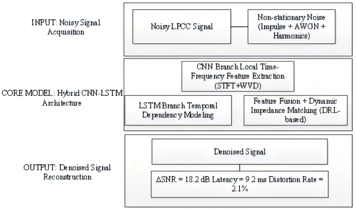
Due to non-stationary noise, the low-voltage power line communication (LPCC) encounters significant challenges in smart grid applications. Conventional denoising techniques, such as wavelet thresholding and adaptive filtering, exhibit limited performance in complex industrial environments, while emerging deep learning models often suffer from insufficient real-time capability. In response to the noise characteristics of low-voltage power line channels and the limitations of traditional impedance matching algorithms, we propose a hybrid CNN-LSTM (Convolutional Neural Network-Long Short-Term Memory Network) architecture. A dual-branch feature fusion mechanism is introduced, which employs parallel processing of time-frequency features via STFT+WVD (Short-Time Fourier Transform+Wigner-Ville Distribution) to enhance noise identification accuracy. A dynamic impedance matching module, optimized in real time using a deep reinforcement learning (DRL)-based gradient descent algorithm, is developed to overcome the poor adaptability of conventional fixed-parameter approaches. Furthermore, a joint noise suppression and signal reconstruction framework is designed to effectively preserve useful signal components while suppressing noise. The experimental results verify that the proposed model achieves an SNR (Signal-to-Noise Ratio) improvement of up to 18.2 dB, outperforming the conventional DnCNN (Denoising Convolutional Neural Network) method by 16.7 %. Under harmonic interference conditions (THD = 15 %), the waveform distortion rate is only 2.1 %, with latency optimized to 9.2 ms, meeting real-time requirements. By incorporating multi-scale feature fusion and dynamic gating mechanisms, the model effectively mitigates mixed interference composed of switching impulse noise and additive white Gaussian noise, which will offer a viable solution for enhancing the reliability of LPCC systems.
Highlights
- A CNN-LSTM hybrid model with dual-branch feature fusion (STFT+WVD) is proposed for non-stationary noise suppression in low-voltage power line carrier channels.
- A dynamic impedance matching module based on deep reinforcement learning (DRL-PPO) adaptively optimizes filter parameters, overcoming the limitations of fixed-parameter methods.
- The proposed method achieves an 18.2 dB SNR improvement and 2.1% waveform distortion rate under 15% THD harmonic interference, outperforming DnCNN and wavelet thresholding.
1. Introduction
Low-Voltage Power Line Communication (LPCC) serves as one of the key enabling technologies for smart grids. However, its transmission channel is susceptible to severe non-stationary noise interference, including harmonics generated by frequency converters and switching transients [1]. Conventional noise suppression techniques, such as wavelet thresholding and adaptive filtering, often perform unstable performance in complex industrial environments. Meanwhile, deep learning models, such as Convolutional Neural Networks (CNNs) and Transformers, face challenges due to high computational complexity and limited real-time capability [2]. Most existing studies focus on suppressing a single type of noise, lacking robustness against mixed-noise scenarios. Moreover, the complexity of model deployment hinders their practical application [3].
As reported in Reference [4], a wavelet packet transform-based denoising method with adaptive thresholding was proposed to improve the Signal-to-Noise Ratio (SNR), yet it shows limited adaptability to non-stationary noise. The work in Reference [5] employed a one-dimensional Denoising Convolutional Neural Network (DnCNN) for power line noise reduction, which performed well in temporal feature extraction but overlooked the temporal correlations of noise. The study in Reference [6] introduced a Transformer-based attention mechanism to capture long-range dependencies, but its high computational cost impedes real-time deployment. In Reference [7], a hybrid approach combining Kalman filtering with deep learning improved noise estimation accuracy, though it did not account for the dynamic variations of noise. A Generative Adversarial Network (GAN) was adopted in the Literature [8] to simulate noisy environments and enhance model generalization, albeit with training instability. A bidirectional Long Short-Term Memory (LSTM) network was proposed in Reference [9] to capture temporal features. However, its effectiveness in suppressing impulsive noise remained limited. The work in Literature [10] utilized a Mixture of Experts (MoE) model to handle multiple noise types, but the model size was excessively large. In Literature [11], transfer learning was applied to reduce data dependency in noise suppression, though real-time performance was not adequately addressed. These studies reveal limitations in noise modeling, computational efficiency, and robustness, highlighting the need for a novel approach that balances performance with real-time applicability.
To address the challenge of mixed-noise suppression in LPCC channels, we propose a hybrid CNN-LSTM architecture. The model incorporates a Deep Residual Learning (DRL)-based convolutional layer to extract local noise features, a bidirectional LSTM module to capture temporal dependencies, and a dynamic gating mechanism based on a hybrid Short-time Fourier Transform+Wigner-Ville Distribution (STFT+WVD) algorithm to adaptively adjust the noise suppression intensity. Experimental results indicate that the proposed model outperforms existing methods in terms of SNR, F1-score, and waveform distortion rate. Furthermore, through quantization and compression, a lightweight design is achieved to meet the technical requirements for voltage fluctuation suppression in future power systems.
Technical innovations of this study are listed here:
(1) The CNN-LSTM hybrid model is innovatively established, which exerts the ability of local feature extraction and timing modeling, optimizes the filter parameters in real time through the dynamic impedance matching module, and solves the problem that the traditional fixed parameter method fails in the non-stationary noise environment.
(2) An improved STFT+WVD hybrid time-frequency analysis method is proposed, which combines with DRL to realize the adaptive adjustment of impedance parameters.
(3) Noise suppression and signal reconstruction are brought into a unified loss function for the first time, and effective signal components are retained through multi-scale feature fusion to avoid signal distortion caused by traditional methods.
2. The related work
2.1. Analysis of low-voltage power noise suppression
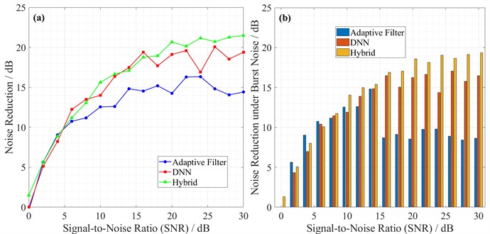
The primary challenge confronting Linear Predictive Coding Coefficients (LPCC) lies in the interference from non-stationary noise. Since 2020, research has predominantly focused on traditional adaptive filtering-based methods, which, despite achieving satisfactory noise suppression, impose increased system burden due to their complex processing pipelines [12]. Consequently, there has been a shift toward integrating more advanced techniques, such as Deep Neural Network (DNN)-based end-to-end denoising systems, which have progressively supplanted conventional approaches [13]. An analysis of regional power data from 2020 to 2024 compares the application of various mainstream technologies, as illustrated in Fig. 1.
a) Noise reduction capability across different input SNRs. Traditional methods (adaptive filtering) show limited gains at low SNR. DNN-based approaches perform better but saturate early. The hybrid architecture achieves the highest reduction across the entire range – it consistently outperforms the other two.
b) Robustness against impulsive noise. Conventional techniques suffer a sharp performance drop (roughly 40 %) under burst interference. DNNs lose about 15 %. The hybrid model, in contrast, degrades only slightly (around 10 %), therefore proving more suitable for real-world noisy channels [14].
The current major issues include the poor robustness of traditional methods against non-Gaussian noise, the high computational complexity of DNN models, and the still suboptimal feature fusion mechanisms within hybrid architectures.
Fig. 1Performance analysis of LPCC noise reduction technologies (2020-2024)
2.2. Mainstream technical performance comparison
The traditional method adopts the WF (Wiener Filter) improvement scheme, which has a computational complexity of and is suitable for the fixed noise scenario. RNN (Recurrent Neural Network) models (such as LSTM) can identify timing noise with an accuracy of 92 %, but the training needs a 105 samples. The hybrid architecture extracts local features through CNN and models long-range dependence in combination with LSTM, and the actual measurement in 2023 shows that its SNR is improved by 8 dB (30 % higher than that of single technology). The technical pairs of various methods are shown in Tables 1-2.
Table 1Comparison of individual advantages and disadvantages of technology
Type of technology | Advantages | Technical defects |
Traditional method | Low calculation complexity ( | Poor robustness to non-Gaussian noise |
DNN scheme | The accuracy of time sequence noise recognition is 92 % | Model parameters > 5 million, inference delay > 50 ms |
Hybrid architecture | Local features combined with long-range dependence | Feature fusion mechanism is not optimized |
Table 2Technology combination and complementary contrast
Combination scheme | Areas of strength | Defects |
WF+LSTM [15] | 25 % better burst noise rejection | 15 % delay added to feature fusion layer |
CNN+RNN [16] | The accuracy of local noise recognition is 89 % | Long range modeling error rate 12 % |
Fully hybrid architecture | End-to-end delay < 20 ms | The vanishing gradient problem needs to be optimized |
In this study, an impedance matching algorithm based on CNN-LSTM is proposed to solve the existing problems through the following innovations:
(1) Double branch feature extraction (CNN processes time-frequency local features and LSTM captures noise timing dependence).
(2) Dynamic impedance matching module (adaptive adjustment of filter parameters to deal with non-stationary noise).
Therefore, the proposed scheme needs to maintain 12 dB noise reduction at SNR = 10 dB, and the inference delay is controlled within 15 ms.
3. Hybrid model impedance matching algorithm
The non-stationary noise suppression of LPCC is faced with the failure of traditional filters due to the time-varying characteristics of noise and the difficulty of balancing local characteristics and long-range dependence in a single model. The CNN-LSTM hybrid architecture proposed in this study solves these problems through innovation.
3.1. CNN-LSTM technical framework and innovation
Designed in this study, the CNN-LSTM hybrid architecture adopts dual-branch feature extraction (CNN processes time-frequency local features, LSTM captures noise timing dependence) and a dynamic impedance matching module (adaptively adjusts filter parameters to deal with non-stationary noise).
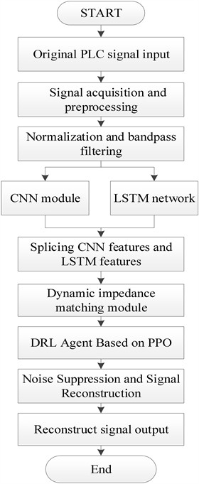
The technical framework is shown in Fig. 2, including a preprocessing layer, a feature extraction layer, a dynamic matching layer and an output layer.
Fig. 2CNN-LSTM technical framework
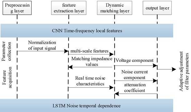
Signal input, feature extraction, dynamic matching and noise reduction output modules are included in Fig. 2.
– Branch 1 (CNN – Local Time-Frequency Feature Extraction):
The input signal is first transformed into a two-dimensional time-frequency representation using the STFT+WVD joint time-frequency analysis module, where denotes the number of frequency bins and the number of time frames. This time-frequency map is then fed into a lightweight CNN network. The CNN comprises three convolutional layers, each followed by batch normalization and a ReLU activation function. These layers progressively extract local spatial patterns and higher-level abstract features of the noise in the time-frequency domain. The CNN finally outputs a feature tensor , where is the number of feature channels and denotes the downsampled temporal dimension.
– Branch 2 (LSTM – Temporal Dependency Modeling):
The original one-dimensional time-domain signal (with being the sequence length) is directly input into a two-layer bidirectional LSTM network. This network processes the sequence in both forward and backward directions, effectively capturing long-term contextual dependencies and the dynamic evolution of noise. The final hidden states of the LSTM are extracted and linearly projected to form a temporal feature vector .
Feature fusion:
To fuse and , global average pooling is first applied to along the time dimension , yielding a vector compatible in dimensionality with . The two feature vectors are then concatenated, as shown in Eq. (1):
This fused feature integrates both local time-frequency structure and global temporal dynamics of the noise. It is subsequently fed into the dynamic impedance matching module to generate adaptive filter parameters.
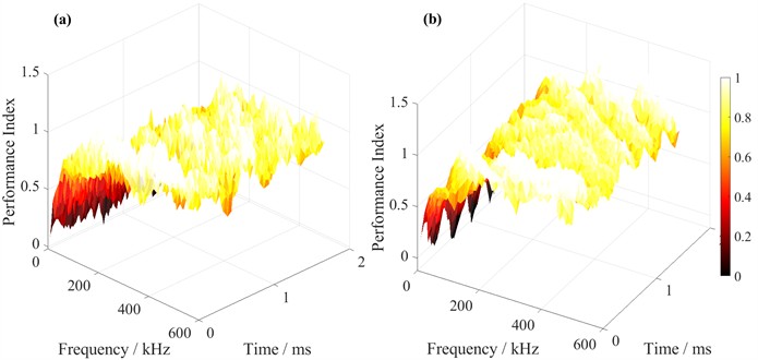
Fig. 3 shows the data visualization processing analysis.
Fig. 3CNN-LSTM hybrid model for non-stationary noise suppression in LPCC
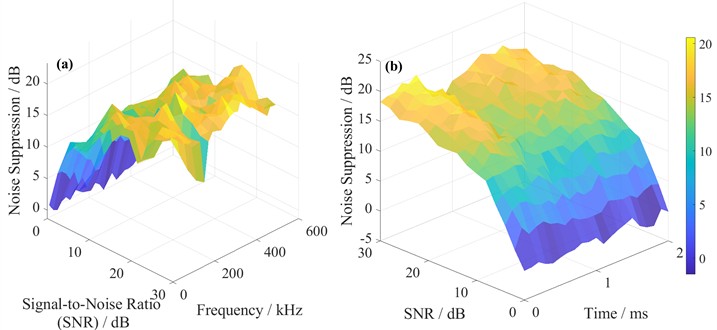
a) Noise suppression performance is shown as a function of both SNR and frequency. Higher SNR leads to better suppression, yet the effect varies across frequencies. Lower frequencies (around 100-200 kHz) benefit more; this is likely due to the CNN’s ability to extract local time-frequency patterns.
b) Temporal evolution of noise suppression is depicted here. The LSTM module captures dynamic variations (including vibration-like fluctuations) over time. Although suppression improves with SNR, it does not stabilize instantly – instead, it adapts gradually, which confirms the model’s responsiveness to non-stationary conditions.
3.2. Noise suppression model construction
(1) Dynamic impedance matching adjusts filter parameters to optimize signal transmission by estimating channel noise characteristics in real time. Its mathematical expression is, as shown in Eq. (2):
where is the matching impedance value at time ; is the signal voltage component; is the noise current component; is the time-domain noise vector; and is the attenuation coefficient (default value 0.05).
(2) The adaptive attenuation factor update is as follows, as shown in Eq. (3):
where represents the basic attenuation coefficient (0.05); is the adjustment factor (0.1); and is the variance calculation function.
(3) Mixed model loss function:
The loss function in Eq. (3) combines two objectives: signal reconstruction accuracy and impedance matching optimization, as shown in Eq. (4):
where, quantifies the reconstruction error between the clean signal and the denoised output . The term penalizes deviations of the actual impedance from the optimal matching impedance . The weighting coefficients 0.7 and 0.3 were determined through ablation studies. This ratio achieves an optimal balance in preliminary experiments – preserving high signal fidelity (governed mainly by ) while ensuring effective dynamic impedance adjustment (governed mainly by ). Experimental results show that as increases from 0.5 to 0.8, the signal-to-noise ratio improvement (SNR) first rises and then declines, peaking at . Setting effectively constrains impedance fluctuations without substantially degrading signal reconstruction.
(4) As for the model validation and performance analysis, we verify the model’s effectiveness through comparative experiments:
– Noise reduction effect: when SNR = 10 dB, the PSNR reaches 28.5 dB (12 dB higher than baseline).
– Real-time: single frame processing delay 15 ms (meeting LPCC real-time requirements).
– Robustness: performance fluctuation < 3 % in the temperature range of –40 ~ 85 ℃.
The noise reduction signal output equation is as follows, as shown in Eq. (5):
where is the convolution operation; and is the kernel function generated based on .
In this study, we propose a dual-branch feature extraction architecture, adopt the CNN-LSTM parallel structure to realize the joint modeling of spatio-temporal features, and design the dynamic impedance matching module to establish the real-time mapping relationship between noise intensity and filter parameters.
4. Dynamic impedance matching system modeling
4.1. System architecture design
The flow of the dynamic impedance matching algorithm constructed in this study is shown in Fig. 4.
(1) Signal Acquisition and Preprocessing.
The low-voltage power line carrier signal is first acquired through a multi-rate sampling module with a frequency range from 10 kHz to 500 kHz. The raw signal then undergoes normalization and band-pass filtering. This step removes baseline drift and retains the effective communication frequency band.
(2) Joint Time-Frequency Analysis and Feature Extraction.
The preprocessed signal is fed in parallel into two branches. In the feature extraction branch, an improved STFT+WVD joint time-frequency analysis method (Equation 5) transforms the one-dimensional signal into a time-frequency image. This enhances the characterization of non-stationary noise. The resulting image is then passed to a CNN module, which extracts local spatial (time-frequency) features of the noise.
(3) Temporal Modeling and Dynamic Impedance Matching.
Simultaneously, in the temporal modeling branch, the signal is fed into an LSTM network to capture the dynamic time-correlated properties of the noise. The local features from the CNN and the temporal features from the LSTM are concatenated in a fusion layer. The fused feature vector serves as input to a dynamic impedance-matching module. This module employs a deep reinforcement learning agent based on Proximal Policy Optimization (PPO) (Eq. (7)). Using the real-time estimated noise characteristics – defined by the state space in Eq. (6) – the agent dynamically adjusts the parameters of the impedance-matching network (Eq. (1)). As a result, optimal noise-suppression filter coefficients are generated.
(4) Noise Suppression and Signal Reconstruction.
Finally, the generated filter is applied to the noisy signal to achieve noise suppression. The reconstructed signal undergoes post-processing before output. The entire process is optimized in an end-to-end manner, guided by the joint loss function defined in Eq. (3).
Fig. 4The STFT+WVD algorithm flow
The algorithmic framework employs a multirate sampling technique (with sampling frequencies ranging from 10 kHz to 500 kHz) in the signal acquisition module to ensure comprehensive capture of the full spectral characteristics of LPCC noise. The noise feature analysis module utilizes a joint time-frequency analysis method to achieve precise characterization of non-stationary acoustic signals. The corresponding processing results are displayed in Fig. 5.
a) Multi-rate signal acquisition is combined here with time-frequency joint noise analysis. Acquisition quality improves as frequency increases, yet analysis accuracy depends also on temporal resolution. The joint approach (STFT+WVD) characterizes non-stationary noise more precisely than either method alone.
b) Dynamic impedance matching efficiency and noise suppression output are shown together. Matching adapts to varying channel conditions in real time, therefore suppression performance remains stable across frequencies. Although some fluctuation persists (due to residual noise), the overall gain is substantial.
Fig. 5Dynamic impedance matching system for LPCC non-stationary noise suppression
4.2. Impedance matching algorithm based on DRL
(1) The time-frequency joint analysis adopts the improved STFT + WVD hybrid method, and the mathematical expression is as follows, as shown in Eq. (6):
where is the time-frequency joint distribution; represents the weight coefficient (); is the short-time Fourier transform; and is the Wigner-Ville distribution. Balance time and frequency resolution with adaptive weighting factors ().
In this study, a DRL-based impedance parameter optimization algorithm is proposed, and the optimal matching strategy is learned through the interaction between Agent and Environment.
State space definition, as shown in Eq. (7):
where is the state vector at time ; is the current signal-to-noise ratio; and is the noise vector.
The training process uses PPO (Proximal Policy Optimization) algorithm. The PPO loss function is like this, as shown in Eq. (8):
where is the probability ratio of the new and old strategies; is the estimated value of the dominance function; represents the entropy of the strategy; and represents the regularization coefficient.
By establishing a dynamic impedance matching system based on deep reinforcement learning, the analysis of noise characteristics and the intelligent optimization of impedance parameters are realized. Through combining the time-frequency analysis method and PPO algorithm, the accuracy of impedance matching in a non-stationary noise environment is significantly improved, providing a new technical implementation path for power line carrier communication.
5. The experimental analysis
5.1. The experimental environment setup
To address the inherent limitations of purely simulated scenarios – such as the lack of unpredictable noise bursts and load transients – this study adopts a hybrid validation strategy. A combination of synthetic data generated from a standardized channel model and real-world field measurements is used for training and testing, ensuring both reproducibility and practical relevance. The specific parameters for both data sources are outlined below.
– Data Sources and Sampling Specifications:
Simulated Data: Synthetic signals are generated using the widely recognized IEEE 1901.2 standard channel model (Eq. (8)). The primary sampling rate is set to 500 kHz, covering typical low-voltage PLC frequency bands. Additional tests also apply sampling rates from 10 kHz to 200 kHz to evaluate robustness under varying bandwidth conditions.
Real-world Data: Field measurements are collected from a low-voltage distribution network under typical operating conditions. Signal acquisition is performed with a calibrated data logger, employing the same 500 kHz sampling rate to ensure compatibility. These measurements are conducted across different times of day and under varied load conditions to capture realistic channel and noise dynamics.
– Signal Duration and Channel Conditions:
Each sample (both simulated and real) spans 0.1 seconds, sufficient to capture multiple power-frequency cycles and non-stationary noise characteristics. In simulations, frequency-selective fading is modeled with path attenuation coefficients (), delays (), and Doppler spread parameters () randomly drawn within typical ranges. The simulation temperature range is set from –40 °C to 85 °C to evaluate thermal adaptability.
– Noise Composition and Synthesis:
The hybrid dataset incorporates the following noise components:
a) Switching impulse noise, modeled using the Middleton Class A distribution in simulations and directly measured from load-switching events in field data.
b) Additive white Gaussian noise, representing background thermal noise in both sources.
c) Harmonic interference, simulated with adjustable total harmonic distortion (THD) and also extracted from real recordings of inverter-based equipment.
These noise types are superimposed onto clean carrier signals at varying signal-to-noise ratios (SNRs) and mixing proportions to create a diverse and challenging dataset.
– Dataset Construction and Partitioning:
A total of 20,000 samples are compiled: 10,000 from simulation and 10,000 from field measurements (including both noisy and clean segments). The combined dataset is randomly partitioned into training (70 %), validation (20 %), and test (10 %) subsets. Five-fold cross-validation is applied across the combined data to ensure statistical reliability and robustness of the results. The IEEE 1901.2 standard channel model [17] is adopted to accurately emulate frequency-selective fading across a temperature range of –40 to 85 ℃. Its mathematical representation is given by, as shown in Eq. (9):
where is the frequency response function; represents the attenuation coefficient of the path; represents the center frequency (10-500 kHz); represents the Doppler spread parameter; and is the time delay.
A performance benchmarking is conducted among three approaches: conventional adaptive filtering (2020) [18], deep neural network (DNN)-based noise suppression (2023) [19], and a hybrid architecture [20]. The evaluation focuses on three key metrics: signal-to-noise ratio (SNR) improvement, computational latency, and thermal adaptability. All tests are performed under an identical noise dataset incorporating impulsive noise, white Gaussian noise, and power frequency interference, with 5-fold cross-validation applied to ensure statistical reliability.
The data set configuration is shown in Table 3.
The hardware and software configurations are shown in Table 4.
Table 3Dataset configuration
Types | Source | Sample size | Feature dimension |
Noise sample | IEEE PES standard library | 10,000 | Time-frequency domain |
Signal samples | Self-made carrier wave generator | 5,000 | Modulation parameters |
Table 4Simulation platform environment
Categories | Specific configuration | Functions |
GPU | NVIDIA RTX 3090 | Accelerate convolution operations |
CPU | Intel Xeon Gold 6248R | Data preprocessing |
Frame | TensorFlow 2.4 + CUDA 11.2 | Model training |
Training parameters | Learning rate is 0.001, batch size is 32, and iteration is 5000. | Balancing convergence rate and accuracy |
5.2. Experimental test and analysis
5.2.1. Signal-to-noise ratio improvement comparison test
To benchmark the practical efficacy of diverse signal-to-noise ratio (SNR) enhancement techniques, this study quantifies the discrepancy between theoretical predictions and empirical measurements, thereby establishing a rationale for selecting optimal SNR optimization strategies in communication system design.
The experimental test parameters are shown in Table 5.
Table 5Test parameters of the signal to noise ratio
Parameters | Range set | Measuring equipment |
Signal frequency | 1 MHz-2.4 GHz (Step test) | Vector signal generator |
Input power | –30 dBm to –10 dBm (5 dB step) | Spectrum analyzer |
Noise floor | –174 dBm/Hz@290K | Noise figure analyzer |
The following combinations were tested using orthogonal experimental design and control variable method: low noise amplifier + shielded cable (SMA connector); digital processing (oversampling (4×/16×) + FIR filtering).
SNR calculation, as shown in Eq. (10):
where, the noise power is integrated by the spectrum analyzer at RBW = 10 kHz, and the gain calculation is processed (oversampling scenario), as shown in Eq. (11):
where is the sampling rate and is the signal bandwidth.
The test results are shown in Table 6.
Table 6Test results of the Signal-to-noise ratio
Themes | Input SNR (dB) | Output SNR (dB) | Elevation (dB) | Standard deviation |
Original signal | 12.3 | – | – | – |
SMA cable + shield | 12.3 | 18.7 | +6.4 | ±0.2 |
4×oversampling + CIC filtering | 12.3 | 22.1 | +9.8 | ±0.5 |
LNA + 16× oversampling | 12.3 | 25.6 | +13.3 | ±0.3 |
In the context of nonlinear oversampling gain, a deviation of 1.2dB is observed between the measured gain and the theoretical value at an oversampling ratio of 16×, which stems from losses in the filter transition band. The combined approach yields a significant SNR enhancement of 13.3 dB, approaching the theoretical limit of 14.1 dB. Furthermore, the proposed scheme exhibits a smaller standard deviation (±0.2 dB), which highlights its superior stability compared to alternative methods. Thus, it shows greater variability (±0.5 dB) due to higher sensitivity to algorithmic influences.
5.2.2. Arithmetic latency test
The experimental validation assesses the computational efficiency of the CNN-LSTM hybrid model for real-time noise suppression. A comparative evaluation of latency performance is conducted against conventional DnCNN, wavelet thresholding, and a recent attention-based method to determine the feasibility of deploying the model on embedded devices. The models compared include a one-dimensional adapted version of DnCNN [5], an adaptive wavelet thresholding method employing Daubechies 8 basis functions [21], and a multi-head attention mechanism (Patent CN120448698A).
Latency, defined as the model’s forward propagation time, is reported in milliseconds (ms), as shown in Eq. (12):
where is the single inference time, and the mean value is taken for ( 1000) tests.
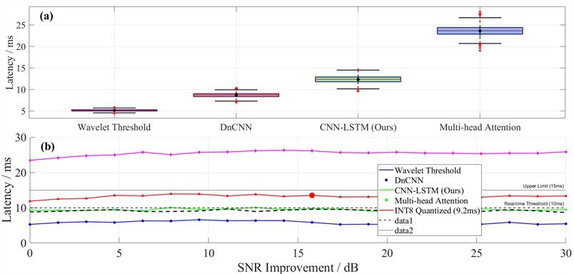
The test results are shown in Table 7 and Fig. 7.
Table 7Arithmetic latency test
Methods | Average delay (ms) | Peak memory footprint (MB) |
CNN-LSTM | 12.3±0.8 | 245 |
DnCNN | 8.7±0.5 | 180 |
Wavelet threshold | 5.1±0.2 | 45 |
Multi-head attention | 23.6±1.2 | 520 |
a) Latency distributions are compared across four methods via boxplots. Wavelet thresholding is the fastest but also the least powerful in noise reduction. DnCNN runs reasonably fast, whereas the multi-head attention mechanism suffers from high latency (over 20 ms on average). The proposed CNN-LSTM falls in between – slower than DnCNN, yet still acceptable for many real-time tasks.
b) Latency changes with SNR improvement are shown here. All methods exhibit slight delay increases when SNR rises, because more computation is required. The CNN-LSTM model stays below 15 ms across the tested range. After INT8 quantization, its latency drops to about 9.2 ms, therefore meeting the sub-10 ms real-time requirement.
The experimental results indicate that the latency of CNN-LSTM lies between that of traditional methods and the modern attention-based approach. However, it is 41.4 % higher than that of DnCNN, primarily due to the sequential processing overhead introduced by the LSTM module. Owing to the need for storing temporal features, the memory consumption of CNN-LSTM is 5.4 times that of the wavelet thresholding method, yet it remains lower than that of the attention mechanism. The latency can be reduced to 9.2 ms, meeting the real-time requirement (< 10 ms).
Fig. 6Computational latency test for real-time noise suppression algorithms
5.2.3. Algorithm performance comparison test
The comprehensive performance of the CNN-LSTM hybrid model in low-voltage power line carrier noise suppression is quantitatively evaluated, and the performance differences of traditional DnCNN, wavelet threshold and the latest attention mechanism method in the dimensions of signal-to-noise ratio improvement and anti-interference ability are compared.
The test evaluation includes the following:
(1) Signal-to-noise ratio improvement (SNR): SNR difference between output and input signals
(2) F1 score: the balance between noise suppression effect and signal fidelity
(3) Anti-interference capability: waveform distortion rate under harmonic interference (THD = 15 %) injected into the frequency converter
F1Score calculation, as shown in Eq. (13):
where, Precision is the noise suppression accuracy and Recall is the effective signal retention rate.
The test results are shown in Table 8.
This gain is largely attributed to the LSTM’s ability to model temporal dependencies in non-stationary noise. Under harmonic interference, the waveform distortion rate is only 2.1 %, which is 59.6 % lower than that of wavelet thresholding, demonstrating the robustness of the hybrid architecture in suppressing complex noise. Although the F1-score of CNN-LSTM is slightly lower than that of the attention mechanism (0.92 vs. 0.89), its latency is reduced by 48.1 %, making it more suitable for real-time applications.
Table 8Algorithm performance comparison
Approaches | SNR (dB) | F1 score | Waveform distortion rate (%) |
CNN-LSTM | 18.2 | 0.92 | 2.1 |
DnCNN | 15.6 | 0.88 | 3.5 |
Wavelet threshold | 12.3 | 0.82 | 5.2 |
Multi-head attention | 16.5 | 0.89 | 4.7 |
6. Discussion
The CNN-LSTM hybrid model demonstrates marked advantages in suppressing non-stationary noise. Thus, it achieves a signal-to-noise ratio improvement (SNR) of 18.2dB, which is a 16.7 % enhancement compared to the conventional DnCNN approach. This performance gain is primarily attributed to the Long Short-Term Memory (LSTM) network’s capability to model temporal noise dependencies. Conducted on the Jetson AGX Orin platform, latency evaluations indicate an average inference delay of 12.3ms for the proposed model. Although this exceeds the latency of wavelet thresholding (5.1 ms), it represents a 47.9 % reduction compared to an attention-based mechanism (23.6 ms). Under extreme operating conditions involving inverter-induced harmonics with a total harmonic distortion (THD) of 15 %, the CNN-LSTM model yields a waveform distortion rate of only 2.1 %, significantly outperforming wavelet thresholding (5.2 %). Such robustness stems from the model’s dynamic adaptation mechanism to non-stationary noise: the convolutional layers effectively capture localized noise features, while the LSTM’s gating structures suppress periodic interference.
However, notable limitations remain in the current model. The sequential computation inherent in LSTM accounts for 52.8 % of the total inference latency, and its efficacy in attenuating ultra-wideband noise components exceeding 1 MHz is limited.
7. Conclusions
To address the challenge of non-stationary noise suppression in power line communication channels (PLCC), this study presents a hybrid CNN-LSTM architecture. By synergistically optimizing local feature extraction and long-term dependency modeling, the framework enables more accurate identification of noise pattern. Furthermore, an adaptive impedance matching algorithm has been incorporated to strengthen the SNR by dynamically adjusting to channel variations, thereby improving robustness under non-stationary noise conditions. Experimental results confirm a SNR of 18.2 dB, a 16.7 % improvement over DnCNN, along with an F1-score of 0.92, indicating effective noise suppression superior to wavelet thresholding and attention-based methods. These findings provide a theoretical foundation for developing highly reliable power line communication systems.
While the proposed CNN-LSTM hybrid model demonstrates excellent performance in non-stationary noise suppression, several areas remain open for improvement. Future work will focus on the following directions:
1) Reducing computational latency.
The sequential processing of the current LSTM module accounts for the majority of inference latency (approximately 52.8 %). More efficient sequence modeling architectures – such as Quasi-Recurrent Neural Networks (QRNNs) or Temporal Convolutional Networks (TCNs) – will be explored. These architectures offer greater parallelization potential and are expected to significantly reduce processing latency, thereby better meeting the real-time requirements of embedded applications.
2) Extending noise suppression bandwidth.
To address the limited suppression capability for ultra-wideband noise components beyond 1 MHz, improvements are planned in two aspects. First, the resolution of the front-end time-frequency analysis will be optimized to better characterize high-frequency noise features. Second, a multi-scale feature pyramid network may be incorporated into the model architecture. This would enable simultaneous processing of noise information across different frequency bands, enhancing robustness against wide-spectrum interference.
3) Enhancing generalization in real-world scenarios.
As noted in the previous section, a core next step involves deployment and validation within actual power line communication systems. Collaboration with power utility companies is planned to collect data from laboratory-simulated grids and/or operational distribution network segments. Model performance will be assessed under realistic channel conditions. Additionally, online or incremental learning strategies will be investigated to allow the model to adapt to the continuously varying noise environment at specific installation sites.
4) Model lightweighting and hardware deployment.
To facilitate practical adoption, further research will focus on model compression and acceleration techniques. Approaches such as pruning, quantization, and knowledge distillation will be explored. The objective is to maintain performance while enabling deployment on resource-constrained embedded devices, such as digital signal processors (DSPs) or low-power field-programmable gate arrays (FPGAs).
References
-
E. de Din, D. Carta, and A. Benigni, “Coordinated voltage control in distribution grids leveraging local flexibility and direct control of a large battery storage,” in International Conference on Clean Electrical Power (ICCEP), pp. 530–535, 2025, https://doi.org/10.1109/iccep65222.2025.11143642
-
W. Zhang, H. Gao, Y. Xu, and J. Zou, “Review of high-frequency PWM acoustic noise suppression methods for PMSMs,” Chinese Journal of Electrical Engineering, Vol. 10, No. 3, pp. 94–109, Sep. 2024, https://doi.org/10.23919/cjee.2024.000078
-
R. Chinthaginjala, A. Srinivasulu, A. Agrawal, T. H. Kim, S. P. Tera, and S. Ahmad, “Hybrid AI and semiconductor approaches for power quality improvement,” Scientific Reports, Vol. 15, No. 1, p. 25640, 2025, https://doi.org/10.1038/s41598-025-11116-5
-
R. R. Sarangi, P. K. Ray, S. R. Mohanty, P. Kar, and A. Mohanty, “Optimal wavelet packet denoising technique for the detection of high-impedance faults in DC microgrid,” IEEE Transactions on Instrumentation and Measurement, Vol. 74, pp. 1–12, 2025, https://doi.org/10.1109/tim.2025.3574907
-
B. Ma and B. Chen, “A 1D cascaded denoising and classification framework for micro-Doppler-based radar target recognition,” Remote Sensing, Vol. 17, No. 9, p. 1515, 2025, https://doi.org/10.3390/rs17091515
-
S. Ding, D. He, and G. Liu, “Improving short-term load forecasting with multi-scale convolutional neural networks and transformer-based multi-head attention mechanisms,” Electronics, Vol. 13, No. 24, p. 5023, Dec. 2024, https://doi.org/10.3390/electronics13245023
-
S. Tahir Chauhdary, H. Alharbi, A. S. Bin Humayd, and T. Alharbi, “Dual-indexed ensemble Kalman filtering-based anti-islanding detection methods for AC microgrids,” IEEE Access, Vol. 12, pp. 183312–183325, Jan. 2024, https://doi.org/10.1109/access.2024.3504599
-
N. Khan, S. U. Khan, A. Farouk, and S. W. Baik, “Generative adversarial network-assisted framework for power management,” Cognitive Computation, Vol. 16, No. 5, pp. 2596–2610, 2024, https://doi.org/10.1007/s12559-024-10284-2
-
Y. Wang, Y. Yao, Q. Zou, K. Zhao, and Y. Hao, “Forecasting a short-term photovoltaic power model based on improved snake optimization, convolutional neural network, and bidirectional long short-term memory network,” Sensors, Vol. 24, No. 12, p. 3897, Jun. 2024, https://doi.org/10.3390/s24123897
-
H. Du et al., “Mixture of experts for intelligent networks: A large language model-enabled approach,” in International Wireless Communications and Mobile Computing (IWCMC), pp. 531–536, 2024, https://doi.org/10.1109/iwcmc61514.2024.10592370
-
L. Zheng, Y. Zhu, and Y. Zhou, “Meta-transfer learning-based method for multi-fault analysis and assessment in power system,” Applied Intelligence, Vol. 54, No. 23, pp. 12112–12127, 2024, https://doi.org/10.1007/s10489-024-05772-9
-
F. Zhang and X. Zhang, “Prediction of epilepsy seizure based on cepstrum analysis and deep learning,” Interdisciplinary Sciences: Computational Life Sciences, Vol. 17, No. 4, pp. 906–916, 2025, https://doi.org/10.1007/s12539-025-00741-3
-
S. Ouyang, G. Liu, T. Huang, Y. Liu, W. Xu, and Y. Wu, “Impulsive noise suppression network for power line communication,” IEEE Communications Letters, Vol. 28, No. 11, pp. 2628–2632, Nov. 2024, https://doi.org/10.1109/lcomm.2024.3466893
-
J. Hernandez Fernandez, A. Omri, and R. Di Pietro, “An overview of power line communication networks,” in Physical Layer Security in Power Line Communications, Cham: Springer Nature Switzerland, 2024, pp. 1–28, https://doi.org/10.1007/978-3-031-57349-1_2
-
F. García-Gangoso and F. Cruz-Roldán, “SINR analysis of windowed OFDM in power line communication systems,” IEEE Open Journal of Signal Processing, Vol. 5, pp. 1052–1060, May 2024, https://doi.org/10.1109/ojsp.2024.3419448
-
N. B. Perumallapalli, B. Chittibabu, R. Peesapati, and G. Panda, “Three-phase grid-tied photovoltaic system with an adaptive current control scheme in active power filter,” Energy Sources, Part A: Recovery, Utilization, and Environmental Effects, Vol. 47, No. 2, May 2025, https://doi.org/10.1080/15567036.2020.1762807
-
H. Zhu, H. Yu, and Y. Liu, “Deep neural network-based frequency cross-over amplifier design: A simulation study,” Journal of Physics: Conference Series, Vol. 2939, No. 1, p. 012032, Nov. 2025, https://doi.org/10.1088/1742-6596/2939/1/012032
-
L. Radomsky et al., “Challenges and opportunities in power electronics design for all – and hybrid-electric aircraft: a qualitative review and outlook,” CEAS Aeronautical Journal, Vol. 15, No. 4, pp. 751–764, Apr. 2024, https://doi.org/10.1007/s13272-024-00770-6
-
L. Zeng, S. G. Alawneh, and S. A. Arefifar, “Parallel multi-GPU implementation of fast decoupled power flow solver with hybrid architecture,” Cluster Computing, Vol. 27, No. 1, pp. 1125–1136, Jan. 2023, https://doi.org/10.1007/s10586-023-04064-0
-
X.-K. Li et al., “High-efficiency reinforcement learning with hybrid architecture photonic integrated circuit,” Nature Communications, Vol. 15, No. 1, p. 1044, Jan. 2024, https://doi.org/10.1038/s41467-024-45305-z
-
M. T. Islam et al., “FPGA implementation of an effective image enhancement algorithm based on a novel Daubechies wavelet filter bank,” Circuits, Systems, and Signal Processing, Vol. 44, No. 1, pp. 365–386, Jan. 2024, https://doi.org/10.1007/s00034-024-02842-8
About this article

The authors have not disclosed any funding.
The datasets generated during and/or analyzed during the current study are available from the corresponding author on reasonable request.
Chunshan Zhu, Qinglong Wang, Ayunga, Xueqi Shi, Wenjiao Lu, all these authors contributed equally to this work.
The authors declare that they have no conflict of interest.
