Nonlinear mathematical model and method of solving the problem of isothermal flow of real fluid in a pipeline with a damper

1. Introduction

Pipeline transportation of target products plays a key role in various industries, including energy, chemical industry and public utilities. Reliable and efficient operation of pipeline systems requires precise consideration of hydraulic and thermodynamic characteristics of the flow, especially in conditions of complex terrain and non-stationary operating modes. One of the current areas in this area is mathematical modeling of non-stationary flows taking into account the forces of resistance, gravity, inertia and the actual properties of the transported liquid.

Problems of unsteady fluid flow have interested mankind since the advent of hydraulic structures: bridges, pipelines and other elements of hydraulic systems. By the beginning of the 20th century, the main theoretical foundations of this area were laid by such outstanding scientists as M. V. Lomonosov, L. Euler and N. E. Zhukovsky [1]. Numerous scientific studies have been carried out within the framework of this topic. Theoretical foundations for modeling the flow of liquids and gases in pipelines were developed by such scientists as Nikuradze, O. Reynolds, G. Schlichting, N. E. Zhukovsky and others. In recent years, numerical methods (including CFD) have been actively developed, allowing for the complex relief of the route, pressure losses, wave phenomena and friction force when modeling non-stationary processes.

It is especially worth noting the work of D. A. Fox [2], who developed graphical algorithms that served as the basis for subsequent numerical methods for analyzing unsteady flows.

In the work of I. A. Charny [3] more complete equations of pipeline transport of real isothermal liquids are presented. A number of methods of linearization of these equations are proposed. Boundary conditions with dampers of different acting factors are formulated. A method of contour integration in the field of complex numbers is proposed and various variants of solving problems based on quasi-one-dimensional equations of pipeline transport of real liquids are analyzed taking into account small deformation of the pipeline wall.

The article [3] examines unsteady fluid flow in short and long pipelines, taking into account pumping stations, valves and pressure stabilizers. Particular attention is paid to the role of stabilizers in preventing hydraulic shocks in short pipelines. The method of characteristics is used to solve quasi-hyperbolic differential equations. The program is implemented in C++, and graphical visualization is performed in Maple.

Research in the field of short pipelines used, for example, in liquid fuel supply systems for rocket engines, was conducted by such scientists as B. F. Glikman, K. S. Kolesnikov and M. S. Natanzon [4-6]. Significant theoretical and practical contributions to solving problems of pressure stabilization in pipeline systems were made by R. F. Ganiev, H. N. Nizamov and E. I. Derbukov [7]. Numerical algorithms for calculating the flow of multiphase fluid in pipelines were presented in the works of E. I. Massa, V. M. Alyshev and others [8].

The article [9] presents a mathematical model for transporting natural gas through pipeline networks with the addition of hydrogen. The model is based on the equations of conservation of mass and energy and also takes into account the operation of compressor stations that compensate for pressure losses. Initially developed for pure natural gas, the model was adapted for hydrogen-gas mixtures using nonlinear optimization in the GAMS environment. Calculations showed that the addition of hydrogen reduces the transmitted power, and the maximum permissible mass fraction of hydrogen is about 6 %.

Despite the significant contribution of the above-mentioned studies to the development of the theory of unsteady fluid motion, many applied aspects of this problem still remain insufficiently studied. In particular, most models do not take into account important factors such as the influence of pipeline relief, transient processes in closed systems of short and long length, pressure instability, and mass flow rate variations over time.

In this regard, this paper considers the problem of modeling an unsteady isothermal fluid flow in a pipeline with a variable height profile. Unlike known works, the proposed model takes into account the real properties of the liquid and gas transported through the pipeline in the air cap. The main objective of the study is to involve nonlinear numerical methods for solving traveling wave equations in studying the dynamics of liquid mass flow rate, pressure, and flow velocity under transient conditions.

2. Statement and mathematical model of the problem

The isothermal state of a liquid in a pipeline with a constant diameter $D$, length $l$, resistance coefficient $\lambda$, variable leveling height of the pipeline axis $y\left(x\right)$, expressed through the slope of the route $\sin \alpha =\frac{dy\left(x\right)}{dx}$, is described by quasi-one-dimensional equations of conservation of momentum and mass according to quasi-one-dimensional equations of conservation and transfer of mass and momentum and the equation of state of a real liquid [1, 2, 8, 22] Eq. (1):

Here and below $\rho \left(x,t\right)$, $u\left(x,t\right)$, $p\left(x,t\right)$ are the average values of density, velocity and pressure of the liquid in the cross-section $x$ at the moment in time $t$; $p_{*}$, ${\rho }_{*}$ – values of pressure and density in the undisturbed state of the liquid; $k$ – coefficient of volumetric compression of liquid. Otherwise, the usual designations for pipeline transportation are used [1, 5, 9, 22].

The initial distributions of velocity and pressure in the relief pipeline are given.

It is necessary to develop a numerical method for solving the problem within the framework of the approach of propagation of counter traveling waves for given laws of change in mass flow at the entrance to the section and at its exit over time, when an air cap is installed at the exit.

The initial condition can be formed both for the task of starting the operation of a section and for the transition process from one operating mode to another according to the mass flow rate of liquid.

In the first variant of the initial condition, the flow velocity is zero Eq. (2):

Then, according to the first and third equations (the equations of conservation and transfer of momentum and the state of the liquid), a unique barometric formula is compiled Eq. (3):

where $p_{\mathrm{\Delta }}=k-p_{*}=\mathrm{c}\mathrm{o}\mathrm{n}\mathrm{s}\mathrm{t}$.

In the second variant of the initial condition, it is assumed that the section operated in a steady state with a constant mass flow rate. Eq. (4):

where and below $f=\pi D^2/4$ – the cross-sectional area of the pipeline.

To determine the initial pressure distribution along the length of the section, we turned to the stationary equation of conservation of momentum Eq. (5) [20, 21]:

Taking $u=\frac{M^0}{f\rho }$, $\frac{d\rho }{dx}=c^{-2}\frac{dp}{dx}$, $\frac{du}{dx}=-\frac{M^0}{f{\rho }^2{c}^2}\frac{dp}{dx}$, we got the equation Eq. (6):

where the notations $c^2=\frac{dp}{d\rho }=\frac{k}{{\rho }_{*}}$, are used $\rho ={\rho }_0\left(1+\frac{p-p_0}{k}\right)$. For $\sin \alpha =\mathrm{c}\mathrm{o}\mathrm{n}\mathrm{s}\mathrm{t}$ an analytical solution to a similar equation, see [14].

Transforming the equations, we arrive at the equation Eq. (7):

To solve Eq. (7), an explicit approximation scheme with a dimensionless step along the length is used $h$, from which we find $p_{i+1}^0$ Eq. (8):

Calculations start from the known value of the pressure at the entrance to the section $p_0^0=p\left(\mathrm{0,0}\right)$.

For a known pressure value, $p\left(x,0\right)$ the initial distribution of the liquid velocity is determined by the formula $u_i^0=\frac{M^0}{f{\rho }_{*}\left(1+\frac{p_i^0-p_{*}}{k}\right)}$, and the density distribution ${\rho }_i^0$ is determined by the Eq. (8) given above.

Testing of the presented method for finding the distribution of density and pressure gave a good result. Comparison of pressure with the results of the barometric formula at $M^0=$0 kg/s showed a deviation of no more than 0.1 Pa (the relative error does not exceed 10^-6).

The boundary condition of the problem for the end of the section is formulated taking into account the real properties of the gas.

A compressor (air blower) is usually connected to the air caps, which are installed on the water pipes of pumping stations, from above. After a certain period of time (for example, one to three months), the compressor is started to pump air into the air cap to the required mass. That is, in our problem, the mass of air $m_g$ in the air cap can be considered constant. Assuming that the values of the gas compressibility coefficient, $z$, the specific gas constant $R_g$ and the gas temperature $T_0$ are constant in the equation of state of a real gas, it is taken as Eq. (9):

where can the mass of air in the air cap be determined Eq. (10):

From here we find Eq. (11):

where $c_g^2=z{R}_g{T}_0$. Considering that the pressure value $p$ applies both to $x=l$ the pipeline cross-section and to the volume of the air cap, a mass balance of the liquid in the cross-section with the air cap is drawn up Eq. (12):

At a constant volume of the air cap $V_{BK}^l=\mathrm{c}\mathrm{o}\mathrm{n}\mathrm{s}\mathrm{t}$, which consists of the volumes of air $V_g^l\left(t\right)$ and liquid $V_f^l\left(t\right)$, the value is determined Eq. (13):

In this connection, the condition with the damper takes the form Eq. (14):

The value of the air compressibility coefficient $z$ for known values of $p$, ${\rho }_g$ and $T_0$ has a variable nature [16-18]. In the work, $z=1$ [23] was adopted.

To compare the obtained condition with the damper, we present a version of the condition obtained by I. A. Charny for an incompressible liquid and using the state of an ideal isothermal gas [1]:

where $V_0$ and $p_0$ are constant values of volume and pressure of air in the undisturbed (initial) state; a $Q_l\left(t\right)$ is the output volumetric flow rate.

3. Method for solving the problem

Let us transform the equations and conditions for the transition to analogs of traveling waves.

By introducing the substitution $\phi =\ln \frac{\rho }{{\rho }_{*}}$, the equations are presented in the form [23]: Eq. (16):

The initial ones are transformed Eq. (17):

and boundary conditions Eq. (18):

From the last system we move on to the system of equations from the analogues of traveling waves [23] $f_1=\bar{u}+\phi$ and $f_2=\bar{u}-\phi$: Eq. (20):

According to the introduced modifications, we transform the boundary conditions.

In the numerical solution of the problem, the algorithm presented in the works [12, 24] was used. In the new version, the numerical algorithm takes into account: the real properties of liquid and gas, as well as the upper relaxation in the numerical scheme.

Discrete coordinates are entered $i=x/h$ in the interval $i\in [0;N_x]$ with a constant step $h=l/N_x$ ($N_x=$1000). The time step was $\tau =l/\left(5000c\right)$.

Due to the use of upper relaxation, a certain order of the sequence of calculations is imposed. First, for $n+1$ the -th time step, the values $f_{1i}^{n+1}$ were found with an increasing index $i=0,\dots ,N_x$, taking $f_{2i}^{n+1}=f_{2i}^n$. Then, with a decreasing index, $i=N_x,\dots ,0$ they were found $f_{2i}^{n+1}$ using the already known values $f_{1i}^{n+1}$.

Let us dwell on each stage of the calculations [10, 11, 13].

We write the condition at the entrance to the section in dimensionless form:

The method for solving this equation using the tangent method is described in [23] and is reduced to recurrent calculations using the formula Eq. (23):

When $\left|F\left({\bar{u}}^{k+1}\right)\right|<10^{-12}$ an approximate value of the input dimensionless velocity is obtained [15, 19].

When $i=1,\dots ,N_x$ using [23] the formula $f_{1i}^{n+1}=\frac{f_{1i}^n+\sigma \left(1+{\bar{u}}_i^n\right)f_{1i-1}^{n+1}+\tau \Phi \left({\bar{u}}_i^n,{\alpha }_i\right)}{1+\sigma \left(1+{\bar{u}}_i^n\right)}$, Eq. (24):

where $\sigma =\tau /h$, $\mathrm{\Phi }\left({\bar{u}}_i^n,{\alpha }_i\right)=-\frac{\lambda l}{2D}{\bar{u}}_i^n\left|{\bar{u}}_i^n\right|-\frac{\mathrm{l}\mathrm{g}}{c^2\sin {\alpha }_i}$.

the newly found values $f_{1i}^{n+1}$ for calculating $f_{2i}^{n+1}$ with decreasing index $i=N_x,\dots ,0$. And we start the calculations from the boundary node $i=N_x$, for which the condition with the damper is specified:

Here we used the notations $s_l=\left[V_{BK}^l+\frac{c_g^2{m}_g^l(k-p_{*})}{p^2(1,\bar{t})}\right]\frac{1}{\tau fl}\left(>0\right)$, ${\bar{M}}_l\left(\bar{t}\right)=\frac{Q_l\left(\bar{t}\right)}{f{\rho }_{*}с}$, ($\tau$– step in dimensionless time).

From the obtained condition, we can find the value $\bar{u}(1,\bar{t})$. To do this, we take into account that the value is known $f_1=\bar{u}+\phi$. Then $\phi =f_1-\bar{u}$ the dimensionless density is defined as $\bar{\rho }=e^{f_1-\bar{u}}$. Taking into account this replacement, the condition approximated by the explicit scheme takes the form:

Let's compose an auxiliary function with respect to $\bar{u}={\bar{u}}_{Nx}^{n+1}$:

To solve Eq. (27), we used the tangent method based on the recurrence formula Eq. (28):

The iterative process according to this formula continues until one of the conditions is met $\left|Е\left({\bar{u}}^{k+1}\right)\right|<10^{-12}$, $\left|{\bar{u}}^{k+1}-{\bar{u}}^k\right|<10^{-12}$.

According to the obtained value, ${\bar{u}}^{k+1}={\bar{u}}_{N_x}^{n+1}$ we find $f_{2N_x}^{n+1}=2{\bar{u}}_{N_x}^{n+1}-f_{1N_x}^{n+1}$ and ${\phi }_{N_x}^{n+1}=f_{1N_x}^{n+1}-{\bar{u}}_{N_x}^{n+1}$, which are used in the calculations $f_{2N_x-1}^{n+1}$.

And for the descending index $i=N_x-1,\dots ,0$ the formula is used Eq. (29):

We use it when $i=N_x-1,\dots ,0$.

Based on the largest and smallest values $V_g\left(t\right)$ for permissible disturbances in the boundary conditions, the volume of the air cap is selected.

4. Discussion of results

Based on the given material, a program for calculating transient processes on an elementary section of a pipeline was compiled. The following values were used in the calculations: section length – $l=$1000 m, section diameter – 0.2 m, resistance coefficient –$\lambda =$0.01, input pressure –$p_{00}=$7.5 МPа, new input pressure – $p_{0t}=$7.5 МPа. The step in length was $l/1000$, and in time – $l/\left(5000с\right)$. A small step in time allowed us to exclude the process of successive approximation for a new time step. A series of calculations were carried out for a horizontal section of the pipeline with and without taking into account the friction force, when the initial and boundary conditions had constant values.

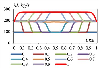
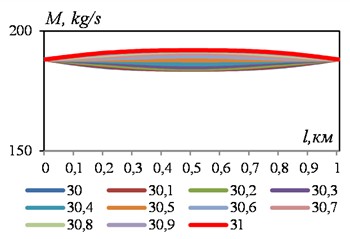
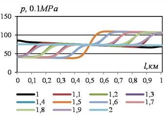
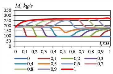
Fig. 1 shows the results of the path change in the mass flow rate of the liquid at different moments in time with a sudden change in the flow velocity at the ends of the section from 3 m/s to 6 m/s. They were obtained at $l=$1000 m, $p_{00}=p_{0t}=$7.5 МPа, $\lambda =$0.01, $D=$0.2 m, $V_{BK}^l=$0 m³.

Fig. 1Path change in the mass flow rate of liquid in some time sections with an abrupt change in flow velocity from 3 m/s to 6 m/s: l= 1000 m, p00= 7.5 МPа, p0t= 7.5 МPа, λ= 0.01, D= 0.2 m, VBKl= 0 m3

a) Left chart

b) Right chart

Fig. 2Temporary change in mass flow rate of liquid in some sections of the section with a sudden change in flow velocity from 3 m/s to 6 m/s. Data see Fig. 1

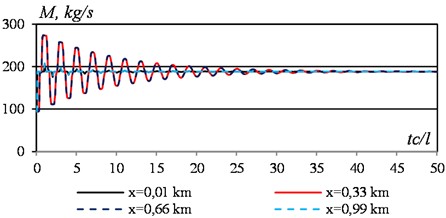
In the first (four after zero) values of time with a step, $T/10=l/\left(10c\right)$ the new mass flow from both ends of the section begins to move toward the middle of the section. When they meet in the middle of the section on the left, the compaction wave and the rarefaction wave on the right first cancel each other out (the graph becomes a straight line), and then new, but smaller values of the mass flow are formed. Subsequently, the upper and lower envelopes of the mass flow curves gradually approach, tending to new values of the boundary velocities. The temporary change in the mass flow of the liquid in some sections of the section shows an exponential damping of the amplitude of the mass flow of the liquid (Fig. 2).

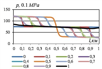
The nature of the pressure change for this calculation option is presented in the following two figures. They demonstrate the types of shock wave with compaction and rarefaction of the transported medium.

Fig. 3Change in pressure along the section at different points in time with increasing flow velocity at the boundaries. Data see Fig. 1

a) Left chart

b) Right chart

c)

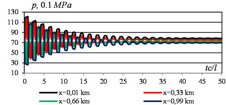
The time changes in the pressure in the sections (Fig. 4) lack the symmetry that was observed in the mass flow graphs. In the last section of time, $(tc/l)$ the values in the four sections of the section were 7.8223, 7.5381, 7.2463 and 6.9528 MPa. At the same time, at the initial moment of the restructuring process, the pressure at the inlet was 7.5 MPa, and at the outlet – 7.27617 MPa. That is, the pressure at the inlet increased, and at the outlet – decreased. And in general, the pressure drop along the section increased, which corresponds to the nature of the object under consideration: an increase in the mass flow rate of the liquid leads to a greater loss of energy.

Fig. 4Temporal changes in pressure in different sections of the section with a two-fold increase in flow velocity at the boundaries. Data see Fig. 1

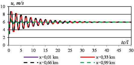
The flow velocity graphs in spatial and time sections are similar in nature to the mass flow graphs, which is due to the relatively small interval of pressure change. In this regard, we will limit ourselves to presenting the time change in flow velocity in different sections. The main changes occur away from the ends of the section.

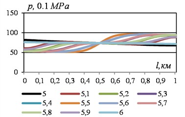
Fig. 5Change in flow velocity in different sections of the pipeline with a simultaneous increase in velocity at the ends of the section from 3 m/s to 6 m/s

The results showed that with a simultaneous change in flow velocity at the ends of a stationary pipeline section, the mass flow graphs are practically symmetrical. Pressure graphs are formed depending on the distance from the beginning of the section. Velocity curves are similar to mass flow graphs.

Similar calculations were carried out for different values of the air cap volume, half of which is occupied by air. Let us dwell on the discussion of the calculation results for the case $V_{BK}^l=$0.01 m³.

Fig. 6 shows graphs of the mass flow rate of liquid along the length of the section for different values of dimensionless time $tc/l$.

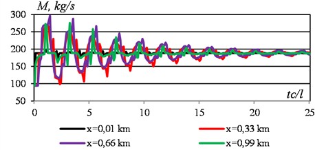
Fig. 6Path change in mass flow rate of liquid in some time sections with a sudden change in flow velocity from 3 m/s to 6 m/s. VBKl= 0.01 m3. For other data, see Fig. 1

a) Left chart

b) Right chart

c) Left chart

d) Right chart

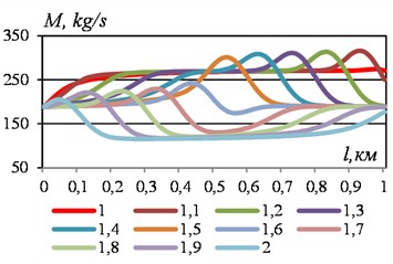
The extreme lower graphs refer to the moment $T/10$. The graph constructed at $tc/l=0$, does not differ from the initial information of the previous calculation option. Also, the left branches of the pressure curves at $\frac{tc}{l}=$0.1, 0.2, 0.3, 0.4 practically repeat the results of the previous option. The presence of an air cap led to the restructuring of the left branches of these pressure curves. First of all, it is striking that the role of the envelopes has lost its force. On the other hand, the boundary value of the mass flow rate of the liquid increases first quickly, and then slowly, and at $tc/l=\text{0.5}$ the level of the average envelope of the left branches is reached. The transition of the pressure curves to such a change in the boundary value of the mass flow rate begins on the right side. Smoother transitions to the initial state are observed at the edges of the rarefaction wave. At $tc/l=\text{0.5}$ the mass flow graph has a spike, as discussed above. But in this case it is significant. At, a spike with a convex graph is formed, which demonstrates the beginning of a rollback of the wave in the opposite direction. The lower parts of the left branches of the graphs are adjusted to the middle envelope, and the upper parts represent a smooth transition. At the right ends of the mass flow curves $tc/l=\text{0.6}$, a slow increase is observed during the time from $tc/l=\text{0.6}$ to $tc/l=\text{0.9}$.

But in the time interval from $tc/l=\text{0.9}$ to $tc/l=\text{1.0}$ the mass flow rate increases abruptly, forming a small spike in the final part of the graph. This spike, firstly, initiates a temporary increase in pressure in the air cap, which leads to a significant local maximum in the mass flow rate profile at $\frac{tc}{l}=$1.1-1.5 (see Fig. 6). Secondly, this spike at the end of the section ends with a decrease in the right end of the graph to the middle envelope during the time interval $tc/l=$1.0-1.1. During the time interval $tc/l=$1.1-1.5 the left branches of the graphs tend to occupy the initial state. Therefore, at $tc/l=\text{1.5}$ the graph in the middle has a single spike with a local maximum.

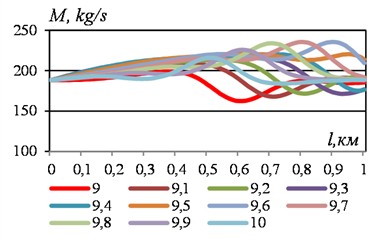
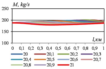
In the next time interval, $tc/l=$ 2.0-3.0 the process is repeated, but with bursts with local minima. That is, we get graphs that are inverted relative to the time interval $tc/l=$ 1.0-2.0. At the same time, the graphs without bursts gradually shorten, and the local maxima and minima are smoothed out (Fig. 6). In turn, zones of close values of mass flow rate and zones with positive and negative bursts of graphs are formed at the left and right ends of the section (Fig. 6). Bursts are also noticeable in the graphs of mass flow rate of liquid, plotted depending on time (Fig. 7). They correspond to the peaks of the red graphs at the bottom and the purple graphs at the top.

Fig. 7Temporal changes in mass flow in different time sections of the section. Data see Fig. 6

Next, we analyze the pressure dynamics for this case.

In the inlet section of the section, the condition of constancy of the mass flow rate of the liquid over time is set. According to this and the equation of conservation of momentum, the derivative of the pressure with respect to the distance at the inlet of the section is zero. Therefore, the pressure graphs at the beginning of the section are perpendicular to the ordinate axis. Such a pattern is also observed in the pressure graphs in the absence of an air cap. In the time interval, $tc/l=$ 0.0-0.5 the left branches of the pressure graphs repeat the nature of the pressure change in the absence of a damper with a jump-like transition to a new pressure value according to the jump in the mass flow rate. The main pressure changes occur in the right branches of the graphs. The rarefaction wave expected at the end of the section is smoothed out due to the softening of the impact by the air cap, which led to a deviation of the graphs from the lower envelope with a slow, rather than a jump-like transition. $tc/l=\text{0.5}$ The graph obtained at shows the general picture related to the time interval $tc/l=$ 0.1-0.5.

Fig. 8Path pressure changes in different time sections obtained with VBKl= 0.01 m3 and simultaneous doubling of the end flow rates of the liquid. Data see Fig. 6

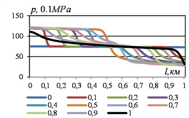
a) Left chart

b) Right chart

Over time, $tc/l=$0.6-0.9 deviations from the middle envelope are noticeable in the right upper branches, and in the left lower branches, features of the graphs characteristic of the case of the absence of an air cap remain. At, $tc/l=\text{1.0}$ maximum deviations from the middle envelope are achieved, especially in the initial sections of the section.

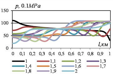
Significant qualitative changes in the pressure graphs occur in the time interval $tc/l=$ 1.0-1.1. At the left end of the graphs, a decrease occurs, which continues to the lower envelope. At the right end of the section, over time, $tc/l=$ 1.0-1.2 the pressure increases to the upper right envelope. A pressure surge is formed, caused by the response of the air cap in the time interval $tc/l=$ 1.1-1.9. It is the reason for the formation of a local minimum in the pressure graph at the beginning of the section at $tc/l=\text{2.0}$. This minimum, as the results showed, is the lowest pressure value in the process under consideration, which was not observed in the absence of an air cap.

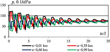
Fig. 9Pressure changes in different sections of the section, obtained with VBKl= 0.01 m3 and simultaneous doubling of the end flow rates of the liquid. Data see Fig. 1

The pressure surge formed by the first wave rollback from the damped end of the section is then always expressed as a local minimum in the graphs.

In the meantime $tc/l=$ 5.0-6.0 The bursts with local minimums move to the right side of the graphs, and in the interval $tc/l=$ 6.0-7.0 – to the left side of the graphs. The parts with pressure bursts gradually decrease.

The nature of the temporary change in pressure in different sections of the section is presented graphically in Fig. 10. It can be seen that the highest value is 121.332 MPa and the lowest, as already noted, is 19.246 MPa. In the absence of a damper, these values were 121.221 and 40.2 MPa.

Calculations carried out for $V_{BK}^l>$ 0.01 m³ showed that with an increase in the volume of the air cap, the transitions in the results become smoother.

5. Conclusions

The computational results demonstrated that a sudden twofold increase in the flow velocity at both ends of the pipeline section generates complex wave dynamics in the transient processes of mass flow rate, pressure, and velocity. In the absence of a damper (air chamber), the mass flow rate profiles are nearly symmetrical, while the pressure distribution is formed depending on the longitudinal distance from the inlet. When a damper is applied, wave attenuation is observed, with sharp variations in pressure and mass flow rate being smoothed, and the amplitude of reflected waves reduced.

The findings indicate that increasing the air chamber volume decreases the difference between the maximum and minimum pressure values, smooths wave processes, and mitigates the risk of hydraulic shock. Furthermore, the location and amplitude of local minima in the pressure–time profiles are significantly influenced by the volume and placement of the damper. These results have practical significance for selecting optimal air chamber parameters to stabilize transient processes and reduce energy losses in pipeline systems.