Abstract
With Europe’s aim for significant renewable energy expansion by 2050, optimizing wind farm performance is critical. This paper investigates the optimization of wind farm layouts using Multi-Rotor (MR) and Single-Rotor (SR) turbines along the Norwegian coast, focusing on the Utsira Nord and Sørlige Nordsjø II sites. The study utilizes Python-based tools, including PyWake and TopFarm, to model and simulate wake effects and turbine performance. MR turbine systems, with their modular configuration, offer advantages in terms of maintenance and uptime. However, SR turbines outperformed MR systems in terms of annual energy production (AEP), yielding at least 11 % more energy. The paper concludes that further optimization strategies, particularly for MR turbines, are needed to realize their full potential, particularly with more advanced wake models and lifecycle cost assessments.
1. Introduction
1.1. Background
In 2020, the European commission presented its strategy for expanding Europe’s renewable offshore energy capacity [1]. As part of the Commission's initiative to make Europe climate neutral by 2050, 300 GW of installed offshore capacity must be realized. In 2020, Europe had a capacity of 12 GW, meaning its current capacity needs to be increased by almost 30 times [1]. In order for Europe to reach this goal, Norway has to dramatically increase its investments in offshore wind energy. In contrast to Norway's thorough experience with offshore oil production, the country is relatively new to offshore wind farms (WF). Currently, the only operational offshore WF in Norway is Hywind Tampen, containing 11 wind turbines (WT) [2]. In 2020, the Norwegian government announced the opening of several sites along the coast for the development of renewable offshore energy [3]. This paper will focus on two of these sites, namely Utsira Nord and Sørlige Nordsjø II.
One of the main issues when designing WFs are the challenges posed by wake effects. Research indicates that wakes induced by WFs could reduce the overall energy production for down-stream WFs by as much as 20 % [4]. This would lead to a substantial reduction in revenue, while possibly disincentivizing further renewable offshore developments. The development of different types of turbine systems poses opportunities for the future of WFs. The concept of MR turbine systems, characterized by floating, vertical arrays hosting numerous smaller turbines, lacks a comprehensive comparison to traditional SR turbines. Despite their potential, the lack of comparison between systems hinders an understanding of their potential advantages.
1.2. Wind turbine types
The two main turbine configurations considered in offshore wind development are single-rotor (SR) and multi-rotor (MR) systems. Each presents unique advantages and challenges, particularly in the context of wake effects and maintenance. This section outlines their core characteristics.
Single-Rotor (SR) Turbines – Horizontal Axis wind turbine Almost all commercial WTs today are built on the horizontal-axis design principle. Like airplane propellers, these turbines usually have either two or three blades, with their axis of rotation parallel to the ground. Its design allows for precise control of the turbine speed via changing the blade pitch [5]. These WTs come in a myriad of sizes with ranging power production capabilities. The blade size of the turbine is the determining factor for the power production [6]. Small-scale turbines often installed on single homes have capacities ranging between 400 Watts and 100 Kilowatts. These typically range in diameter between 1 and 15 meters. On the other end of the spectrum, the largest commercial-scale turbines can currently reach diameters of 240 meters with capacities up to 15 Megawatts [6], [7]. Assuming optimal wind conditions, one of these turbines could generate enough power annually to supply over 4 500 Norwegian households [8]. Fig. 1 shows a typical configuration as well as the main components of HAWTs.
Fig. 1Diagram of the main parts and components of HAWTs [9]
![Diagram of the main parts and components of HAWTs [9]](https://static-01.extrica.com/articles/25071/25071-img1.jpg)
Multi-Rotor (MR) Turbine Systems MR turbine systems is an innovative alternative to the classic SR turbines. Instead of each turbine operating as a stand-alone unit, MR systems contain many smaller rotors in a cohesive framework [10]. SRs have large rotor blades which makes it possible to capture large amounts of energy. The alternative solution posed by MRs is the collective power generation of multiple smaller rotors in a system, making up for their reduced individual power output. Companies specializing in MR technology are working on improving their designs and making them a realistic option to SRs. The improvements aim to extenuate up-time and simplify maintenance, thereby making them a cost-effective alternative to SRs [11]. This would strengthen the prospect of the MR as a promising alternative within the renewable energy sector.
The Windcatcher provides remarkable efficiency, where five units would be capable of generating the same amount of electricity as 25 SRs. This efficiency stems from the strategic grid-like positioning of the turbines [12]. A notable advantage in the Windcatcher design is its maintenance efficiency. With SRs, maintenance typically results in a complete halt in energy production, potentially causing the turbine to remain offline for months [11]. In contrast, the setup for the Windcatcher allows for targeted maintenance where only the affected rotor would need to be offline [11].
Fig. 2Digital rendering of the “Windcatcher” at sea [16]
![Digital rendering of the “Windcatcher” at sea [16]](https://static-01.extrica.com/articles/25071/25071-img2.jpg)
The remaining turbines would continue their operation, leading to more consistency in energy production and minimizing revenue losses related to downtime [12].
The Windcatcher also offers another advantage: it eliminates the need for a specialized watercraft. This is because the Windcatcher has its own self-contained maintenance infrastructure [13]. In contrast, the longer downtime of SRs is mainly caused by their larger rotor sizes, making them require specialized transportation and caution [11]. The smaller rotors of wind-catching systems not only facilitate transportation, but also contribute to decreased downtime, thereby enhancing their overall logistical efficiency [12].
Vertical-Axis Wind Turbines: Vertical-axis WTs (VAWTs) are WTs that rotate their airfoil blades about a vertical axis. These turbines predate the conventional and horizontal propeller-style turbine by over 1000 years, with evidence of construction being found in ruins dating back to 200 BCE in Persia [14]. The two most common types of VAWTs use either the Darrieus or the Savonius airfoils (see Fig. 3), which are drag-driven and lift-driven, respectively [14]. Due to the limited output of drag-driven turbines, lift-driven designs have seen the most commercial use [14].
Fig. 3Illustration showing the most common VAWT types [14]
![Illustration showing the most common VAWT types [14]](https://static-01.extrica.com/articles/25071/25071-img3.jpg)
VAWTs have not seen the same technological advancements as their horizontal counterparts. The main problem with VAWTs is that they have been unsuccessful at matching the overall efficiency and power output of traditional HAWTs. Their strongest feature is that they do not need to be oriented in the wind direction to work optimally. In addition, due to the fact that the axis of rotation is much closer to the center of gravity they are generally more stable [14]. Due to their comparatively smaller footprint and different wake effects, VAWTs can be placed much closer together, allowing for a greater overall power density [15].
1.3. Objectives
The aim of this paper is to compare the optimized layouts of SR and MR systems based on AEP at Sørlige Nordsjø II and Utsira Nord. To achieve this main objective we have accomplished the following sub-objectives:
1) Construct the MR object in python.
2) Optimize the WF layouts.
3) Conduct a comparison of the AEPs for MR and SR configurations.
2. Methodology
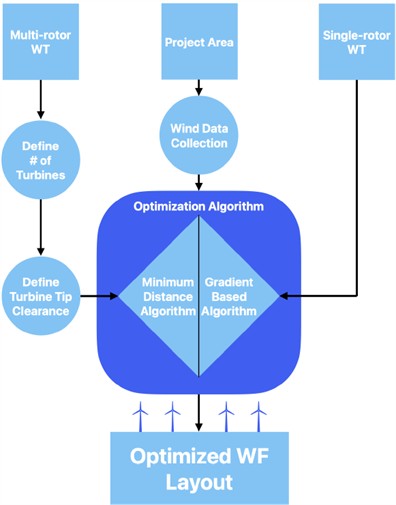
The flow chart of methodology has been shown in Fig. 4. Before we delve into details of the methodology, some assumptions made during this research are:
1) MR wake has been modeled using the Jensen/Park model.
2) The thrust coefficients and power curves for the MR turbines are equivalent for all the optional turbine diameters.
3) The wind conditions are equivalent at all points within the respective project areas.
4) The shear wind is neglected, meaning the wind is equivalent at all turbine heights.
5) The turbulence intensity for all cases is assumed to be 0.1.
The various steps in the methodology are explained below.
Fig. 4Flow-chart of the methodology
2.1. Constructing the wind site object
In order for the optimization task to be accurate and valid, the wind conditions at each of our sites was modeled using meteorological data from NASA’s Earth Science Division Applied Sciences Program [16]. Upon running performwindanalysis.py [17], the script records the input for selecting which geographical area to analyze and uses the integrated Data Access Viewer Enhanced tool (DAVe) to retrieve daily wind data, spanning the past five years. The Wind Speed and Wind Direction at 50 meters above sea level are selected as parameters before retrieving the data as a CSV file. The file is then formatted and sorted for further processing.
Once the CSV data has been correctly formatted, a wind rose is then constructed and plotted. Subsequently, the average wind speeds are calculated and graphed according to a Weibull Distribution. Python’s built-in Weibull function is utilized to fit the data based on relative probabilities. Afterwards, both the wind speeds and their corresponding relative probabilities are presented in the form of Weibull shape and scale factors. The wind speeds are further categorized according to the wind sector they originate from. A total number of twelve sectors was chosen, making each sector 30 degrees wide. Then, applying the Weibull fit function to data from each sector yields Weibull factors for each corresponding wind sector. The number of wind instances in each sector is divided by the total number of instances to produce sector frequencies.
2.2. Optimization
For simulating wake effects, we have used PyWake. Wake modeling has been done using the Jensen/Park model [18]. TopFarm was used for optimizing the SR WF layouts [19]. The functionalities of both PyWake and TopFarm will be explained more thoroughly in Section 2.3 and 2.4.
The objective function we are trying to maximize given the spatial constraints of our sites is the AEP function. This function is defined as follows [20]:
The variable represents the probability of occurrence of each wind instance. represents the sum of the power output from all WTs for a specific wind instance. Wind data is converted into 540 instances. The scalar in front converts the power output to GWh/year, which is a common measurement of power production.
2.3. Understanding PyWake
Site Object and Wind Turbine Object. An important component of PyWake is the site object. The site object defines the wind speeds and their respective probabilities from each direction, like a wind rose. There are three different site classes available to define our site. These are UniformWeibullSite, WaspGridSite and XRSite [18]. Four parameters used to define the site object are the Weibull scale parameter, the Weibull shape parameter, the sector frequency, and the turbulence intensity [18]. The main parameters of the WT object are the thrust coefficient, the power curve, the turbine diameter and the hub height [18].
Modeling Wind Farms The coordinates of the WTs are the only parameters necessary for modelling a WF layout. The layout is modeled by defining a list of -coordinates, -coordinates, and optionally another one for -coordinates. If the -coordinate list is not defined, the height of the turbines will be set to a predefined hub height. All the turbines in a WF are assigned to an index of these lists.
Wind Farm Simulation After defining the site object, WT object, and the and coordinates for the turbines, the WF’s AEP can be simulated. Different sets of turbine coordinates give different values of AEP as a consequence of the wake effect.
2.4. Single-rotor WF optimization
Optimization With TopFarm TopFarm is a Python module Developed by DTU Wind Energy. One of its functionalities is optimization of WF layouts. The TopFarm package can utilize different wake models for flow simulations [19]. OpenMDAO is an open-source platform with Python-based optimization tools for engineering problems. Within OpenMDAO’s library are optimization drivers. The driver serves as a computational tool for finding the most optimal solutions for a given problem [19]. In essence, it is an object that includes instructions for various optimization procedures. The driver most commonly used in TopFarm is called EasyScipyOptimizeDriver [19]. The default algorithm utilized by this driver is Sequential Least Squares Quadratic Programming (SLSQP), which is a gradient-based optimization procedure [19].
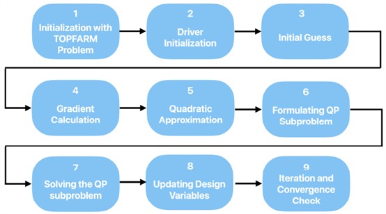
Gradient-based Optimization Gradient-based optimization can be explained using the landscape analogy as done in [21]. To optimize the layout of a WF, it is essential to define the design variables and the objective function accurately. The design variable vector has 2 variables, where represents the number of turbines in a WF. and represents the and coordinate of the th turbine in the WF:
The objective function represents a 2 dimensional landscape of the AEP, and is a function of the design variable vector . The objective function is defined by the PyWake module PyWakeAEPCostComponentModel. The AEP is calculated by Eq. (1):
Subsequently, the gradient of is calculated in Eq. (4) and utilized to minimize the objective function . The gradient represents the direction of steepest decent in the 2 dimensional landscape. Fig. 5 demonstrates the steps involved in the gradient based optimization process:
2.5. Multi-rotor WF optimization
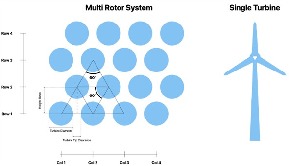
Considering there is currently no template for modelling MRs in PyWake, a variety of relations must be defined. MRs are in simple terms organized groups of many SRs. The SRs are defined in PyWake by their , and coordinates. Therefore, relations between , and coordinates are defined to group SRs into MRs. By writing a function we can automatically output the , and coordinates of all the turbines in MRs. The inputs are the systems center coordinate, its number of rows and columns, the turbine diameter, and the turbine tip clearance. In accordance with the design by Wind Catching Systems AS, we model the turbines to be in a triangular grid with a 60 degree offset between turbine rows, as shown in Fig. 5.
Fig. 5Step-by-step summary of gradient-based optimization process
Minimum Distance Multi-Rotor The minimum distance between MR systems is defined in minimumDistance.py [17]. The wind conditions and the number of rows and columns are taken as inputs, and the minimum distance is returned. First the wind sector with the largest mean wind speed is detected and set as a reference for the following AEP calculations. Before the algorithm runs, the total AEP of two MR systems 20 km apart is calculated. This serves as the reference AEP when the effects of wakes are negligible. Subsequently, we loop through the following calculations.
Fig. 6Simple illustration of the MR system showing configuration and scale
Initially, we calculate the AEP for two MR systems positioned 100 meters apart. The distance is then increased in 100-meter increments, calculating the AEP after each step. We continue this process until one of the following conditions are met: The AEP reaches 99 % of the reference AEP, or the last iteration fails to yield an additional GWh of AEP. When either of these conditions are met, the current distance is returned as the minimum. The reasoning behind the last condition is that we assume that a hundred meters of added distance requires an additional hundred meters of power cable. Installation of a 100 meters of sub-sea power cables cost around 100 000 pounds [22]. Also, we assume an electricity price of approximately 100 000 pounds per GWh [23]. Mathematically, increasing the minimum distance of 100 meters will still be profitable if it results in at least one additional GWh of AEP.
In multiRotorPosition.py the coordinates for the MRs are defined [17]. The inputs are the number of MRs, the outer boundary of the map and the minimum distance between each system. Every MR system will be added to the map incrementally. Each new coordinate has to meet specific conditions to be allowed. First, the distances between the new candidate MR and all previously added MRs must exceed the minimum distance defined previously. Furthermore, an inspection ensures that the candidate MR lies within the boundaries of the map. If the candidate fails to meet either of these conditions, it is discarded, and a new coordinate point is generated.
3. Case study
The chosen MR system design parameters are 5 rows with 5 columns, rotor diameter of 30 meters, and a turbine tip clearance of 1 meter. The wind data and the results for the optimized WT positions are sorted by project area. The results for Sørlige Nordsjø II and Utsira Nord are presented after the WTs objects have been defined.
3.1. Defining wind turbine objects
Single-Rotor Turbine When modeling the SRWT, the IEA Wind 15-Megawatt Offshore Reference WT is used as a reference [7]. The turbine has a power rating of 15MW, cut-in speed at 3 m/s, rated wind speed at 10.59 m/s, and cut-out speed of 25 m/s. The diameter of the turbine is 240 meters, and the hub height is 150 meters [7].
Multi-Rotor Turbine Specific power and thrust coefficients for the individual WTs in our MR system are inspired by the Mitsubishi MWT-1000 turbine. It has a power rating of 1 MW, cut in speed at 4 m/s, rated wind speed at 13.5 m/s, and cut out wind speed at 25 m/s and has a diameter of 57 meters [24]. In reality, MR WTs could have varying diameters depending on its design. We currently assume the power and thrust properties for all prompted diameters to be equivalent to the MWT-1000’s properties.
3.2. Results from Sørlige Nordsjø II
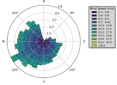
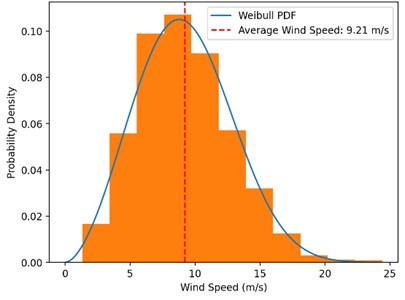
The wind rose in Fig. 7, shows that the wind most commonly originates from the southwestern quadrant. The wind has the lowest probability of originating from the northeast direction. The probability distribution graph shows that the mean wind speed is 9.21 m/s, with a relative probability of occurrence of about 10 %. The shape of the distribution curve shows higher probabilities for speeds close to the mean and decreasing probabilities for higher or lower speeds.
3.2.1. Single-rotor turbines at Sørlige Nordsjø II
In accordance with SNII's established capacity of 1500 MW, we used 100 SRs rated at 15 MW each. After 428 iterations, we obtained a maximum total AEP of 8077.93 GWh. Fig. 8 shows the far (left) and detailed (right) view optimized positions of the turbines, and Fig. 9 shows the AEP development. The detail view shows a marked clustering towards the eastern side of the map, and some minor voids located at the west end, center, north, and south of the project area.
Fig. 9 shows that for a total of 428 iterations the AEP increased by 1.22 %. Specifically, the resulting layout yields 1.22 % better AEP than random positions. We observed a rapid increase throughout the first hundred iterations with a growth from around 7980 GWh to about 8045 GWh. From iteration 100 to around 260, the growth became slower, but still increased to approximately 8070 GWh. The remaining 150 iterations experienced a stagnation in growth, producing an additional 7 GWh.
Fig. 7Illustrations showing the wind conditions at Sørlige Nordsjø II
3.2.2. Multi-Rotor Systems at Sørlige Nordsjø II
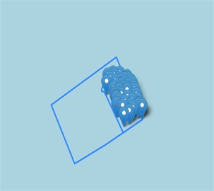
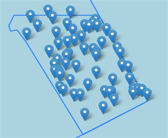
Utilizing the selected parameters for MRs, 60 systems containing a total of 1500 WTs rated at 1 MW each met the capacity requirements for the area. This configuration yielded a maximum AEP of 7002.23 GWh. The resulting AEP for MRs is 13,2 % lower than the SR counterpart. Fig. 10 shows the final locations of each MR system. In contrast to the SR results, where there is clustering in the east portion of the map, multiple MRs are aligned from the southwest to the north. Large open spaces are present in the northwest and southeast. The cluster line is parallel with the frequent winds coming from southwest, based on the wind rose in Fig. 7.
Fig. 8Map displaying the optimized SR locations for SNII
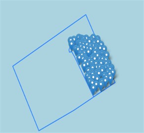
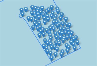
Fig. 9Graph illustrating the improvement in AEP over the course of optimization iterations
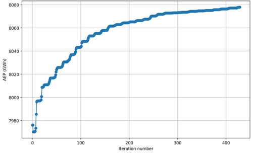
Fig. 10Map displaying the optimized MRS locations for SNII
3.3. Results from Utsira Nord
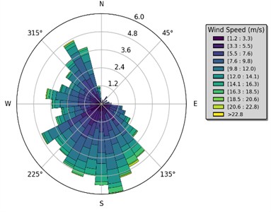
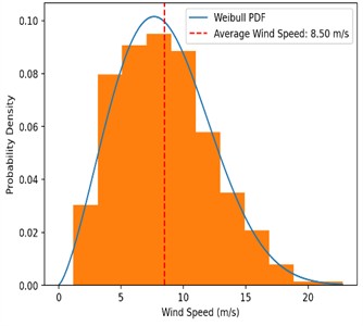
As seen in the wind rose, the wind has the highest probability of originating from the southern region. The wind has the lowest probability of originating from the north and east directions. The probability distribution graph shows the wind speed being centered around 8.50 m/s, occurring about 9.5 % of instances. As previously observed in the probability distribution graph for SNII, wind speeds surrounding the average speed experienced a similar spread, slightly tending towards the lower end of the spectrum.
Fig. 11Illustrations of the wind conditions at Utsira Nord
Single-Rotor Turbines at Utsira Nord Our simulation produced a total AEP of 2436.94 GWh. Since the project area’s capacity is 500 MW, we employed 33 turbines rated at 15 MW. Fig. 12 shows the optimized position of each WT, while Fig. 9 shows the AEP development.
Fig. 12Map of optimized SR layout at Utsira Nord
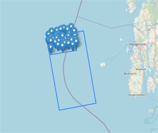
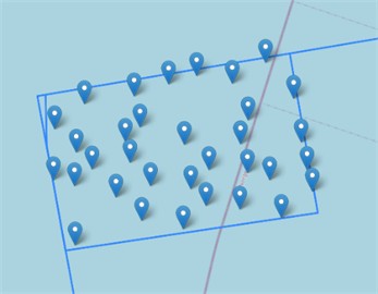
Fig. 12 shows both a far view and a detailed view of the turbine locations. There is an open space on the southwest side of the map. Another open space is present in the central northern edge. Several turbines also appear to be clustered around a diagonal, stretching from the southeast to the northwest.
Fig. 13Graph illustrating the improvement in AEP at Utsira Nord over the course of optimization iterations
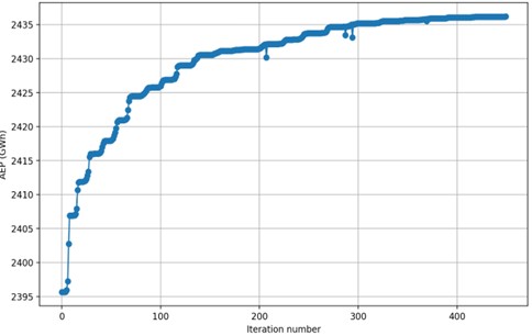
The AEP for Utsira Nord experienced a growth of 1.75 % throughout 450 optimization iterations. Specifically, the resulting layout yields 1.75 % better AEP than random positions. The graph shows an initial rapid growth before seemingly plateauing after about 300 iterations. During the first 100 iterations the AEP grew from 2395 GWh to approximately 2426 GWh. Between iterations 100 and 300 the growth became slower but continued to rise to 2435 GWh. The remaining 100 iterations experienced significant stagnation and produced one additional gigawatt-hour of AEP.
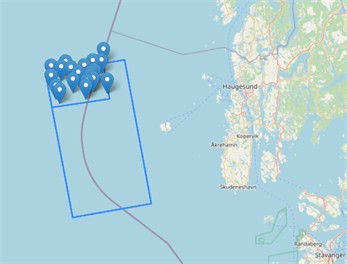
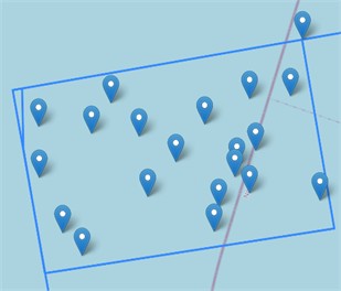
Multi-Rotor System at Utsira Nord The selected parameters for MRs resulted in 20 systems at UN. This includes 500 WTs rated at 1 MW each. The simulation yielded an AEP of 2175.13 GWh. The resulting AEP for MRs is 10.8 % lower than the SR configuration. Fig. 14 show the location of each MR system.
In left part of Fig. 14 we see a far view of the MR system locations at UN. While right part shows a detailed view where a large open space is present in the south-west. Additionally, multiple MR systems cluster in a line from the southeast, stretching north.
Fig. 14Map displaying the optimized MR locations for UN
3.4. Result discussion
Despite SNII’s expected AEP of 7000 GWh, our SR-simulations yielded a total of 8077.93 GWh, while the MR systems yielded 7002.23 GWh. Furthermore, the expected AEP for UN was 2000 GWh. Like before, our simulated AEP using either turbine configuration surpassed this, producing a maximum AEP of 2436.94 GWh and 2175.13 GWh for the SR and MR systems, respectively.
When optimizing the turbine positions, similar outcomes were observed for both project areas. SR turbines consistently outperformed the MR systems, yielding at least 11 % more AEP every time. A notable observation is that the maps of the turbine layouts all contain distinct clusters and voids. The SR position layout for SNII includes a cluster that follows the eastern border of the area. The reason for this occurrence is likely related to the wind conditions. As we discovered, the wind at SNII usually originates from the south/southwest area. The resulting configuration likely originates as a result of minimizing the overall wake interactions.
Regarding the MR layout at SNII, a cluster of systems stretch from the south-west to the north-east part of the area. This cluster would result in unfavorable wake effects on a large portion of the systems. In addition, there is a void in the south-west corner of the project area. There seems to be an imbalance in the placement of systems, meaning our optimization strategy did not work.
The SR layout at UN seems evenly scattered, although this area contains far less WTs than SNII. In contrast to SNII, the MR layout also seems to be evenly distributed, except for a slight cluster to the east of the center. This could potentially explain why the AEP for the MR layout at UN more closely aligned with the results for the SR layout. We believe the minimum distance strategy may have been insufficiently defined. This might be the reason for the unfavorable positioning of the MRs at SNII. As for the resulting AEP deficit, the income loss could be compensated for with the MR system’s highly efficient maintenance procedures and minimized downtime, as described in Section 1.2.
4. Conclusions
This paper examines the comparison of the optimized layouts of SR WTs and MR systems based on AEP, at Sørlige Nordsjø II and Utsira Nord. MRs were successfully modelled in PyWake, before various optimization strategies were tested. Two conclusive optimization algorithms were used to design WF layouts for SRs and MRs. The layouts were then simulated, before the results were compared. The first optimization algorithm we tested was a genetic algorithm, but it was too computationally expensive. Then, a gradient based algorithm was implemented for SR layout optimization. For MR layout, an optimization strategy based on the minimum distance was constructed and implemented. Based on our revised optimization strategies we discovered that the resulting AEPs for SRs exceeded our MR configuration for all cases. In addition, the AEP for both project areas exceeded preliminary estimates, with the exception of MRs at SNII. However, these results do not provide a conclusive comparison of the WT systems. The reason for the inconclusive comparison is likely due to the minimum distance strategy being insufficient, since each test with equivalent inputs resulted in large differences in AEP. In addition, both WT configurations were simulated using the Jensen/Park model, which is primarily designed for modeling SR wakes. Furthermore, the power curves and thrust coefficients for the MR WTs were equivalent for all turbine diameters. In reality, we know these parameters are determined by the rotor diameters, meaning our model was not fully developed.
To conduct a more comprehensive comparison, the minimum distance strategy would need to be revised. In addition, testing more nuanced wake models would improve the study’s real-world applicability. The examination of several optimization algorithms would give more grounds for comparison. Lastly, while the basis for comparison in this paper was the AEP, a more balanced comparison should focus on the LCOE, given that the main advantage of MR systems is their enhanced maintenance procedures. Implementing these changes would offer MR systems a fairer basis for comparison, thereby contributing to the rapidly evolving renewable energy sector.
References
-
“Communication from the commission to the European parliament, the council, the European economic and social committee and the committee of the regions, An EU strategy to harness the potential of offshore renewable energy for a climate neutral future.” Climate Change and Law Collection, European Commission, 2025, https://eur-lex.europa.eu/legal-content/en/txt/?uri=com%3a2020%3a741%3afin
-
“Hywind Tampen.” Equinor, 2019, https://www.equinor.com/energy/hywind-tampen
-
“Norway opens offshore areas for wind power.” Solberg’s Government, Ministry of Petroleum and Energy, 2020, https://www.regjeringen.no/no/dokumentarkiv/regjeringen-solberg/aktueltregjeringensolberg/oed/pressemeldinger/2020/opner-omrader/id2705986
-
E. Finserås, I. Herrera Anchustegui, E. Cheynet, C. G. Gebhardt, and J. Reuder, “Gone with the wind? Wind farm-induced wakes and regulatory gaps,” Marine Policy, Vol. 159, p. 105897, Jan. 2024, https://doi.org/10.1016/j.marpol.2023.105897
-
M. R. Patel and O. Beik, “Wind and solar power systems: design, analysis, and operation,” Choice Reviews Online, Vol. 43, No. 6, pp. 43–3410-43-3410, Feb. 2006, https://doi.org/10.5860/choice.43-3410
-
“Breezing through the basics: Residential wind turbines.” Perch Energy, 2022, www.perchenergy.com/blog/energy/residential-wind-turbines-at-home
-
E. Gaertner, J. Rinker, and L. Sethuraman, “Definition of the IEA wind 15-megawatt offshore reference wind turbine,” National Renewable Energy Laboratory, Technical University of Denmark and University of Maine, Mar. 2020.
-
“Energy consumption in households in Norway.” Statistics Norway, 2021, www.ssb.no/en/statbank/table/11563
-
N. Bagalkot, J. Jose, and A. Keprate, “Key components of the horizontal axis wind turbine,” Multiphysics of Wind Turbines in Extreme Loading Conditions, pp. 17–31, Jan. 2024, https://doi.org/10.1016/b978-0-323-91852-7.00006-4
-
Jan Bartl, “Multi rotor wind turbine designs,” UIB, 2021.
-
I. Knutsen, “Personal communication,” 2024.
-
“Windcatcher with multiple turbines.” Designbloom, 2023, www.designboom.com/technology/floating-wind-power-windcatcher-multiple-turbines-03-15-2023
-
Windcatching. www.windcatching.com
-
R. Whittlesey, Wind Energy Engineering. Elsevier, 2023, pp. 185–202, https://doi.org/10.1016/c2021-0-00258-3
-
J. O. Dabiri, “Potential order-of-magnitude enhancement of wind farm power density via counter-rotating vertical-axis wind turbine arrays,” Journal of Renewable and Sustainable Energy, Vol. 3, No. 4, Jul. 2011, https://doi.org/10.1063/1.3608170
-
P. Stackhouse Jr. et al., “Supporting energy-related societal applications using NASAs satellite and modeling data,” in IEEE International Symposium on Geoscience and Remote Sensing, pp. 425–428, Jul. 2006, https://doi.org/10.1109/igarss.2006.113
-
J. Aarstein, R. K. Aboujamous, J. B. Hagen, and T. Sienes. “Bachelorpapermain,” 2024, https://www.github.com/jonasbryde/bachelorpapermain
-
M. Pedersen, A. M. Forsting, and P. van der Laan. “Pywake 2.5.0: An open-source wind farm simulation tool,” 2023, https://topfarm.pages.windenergy.dtu.dk/pywake
-
R. Riva, J. Y. Liew, and M. Friis-Møller. “Welcome to topfarm,” 2018, https://topfarm.pages.windenergy.dtu.dk/topfarm2/index.html
-
“Windfarm layout optimisation challenge.” Shell, 2020, www.shell.in/energy-and-innovation/ai-hackathon/_jcr_content/par/textimage_1834506119_1619963074.stream/1612943059963/4b0a86b7cc0fe7179148284ffed9ef33524c2816/ windfarm-layout-optimisation-challenge.pdf.
-
S. Ruder. “An overview of gradient descent optimization algorithms,” 2016, https://www.ruder.io/optimizing-gradient-descent/.
-
K. Nieradzinska, C. Maciver, S. Gill, G. A. Agnew, O. Anaya-Lara, and K. R. W. Bell, “Optioneering analysis for connecting Dogger Bank offshore wind farms to the GB electricity network,” Renewable Energy, Vol. 91, pp. 120–129, Jun. 2016, https://doi.org/10.1016/j.renene.2016.01.043
-
N. Ford. “Offshore wind price hike set to revive UK decarbonization goal,” 2024, www.reuters.com/business/energy/offshore-wind-price-hike-set-revive-uk-decarbonisation-goal-2024-02-15.
-
H.-G. Kim and J.-Y. Kim, “Analysis of wind turbine aging through operation data calibrated by LiDAR measurement,” Energies, Vol. 14, No. 8, p. 2319, Apr. 2021, https://doi.org/10.3390/en14082319
-
“Mitsubishi MWT-1000,” 2024, https://en.wind-turbine-models.com/turbines/608-mitsubishi-mwt-1000.
-
J. S. Touma, “Dependence of the wind profile power law on stability for various locations,” Journal of the Air Pollution Control Association, Vol. 27, No. 9, pp. 863–866, Sep. 1977, https://doi.org/10.1080/00022470.1977.10470503
-
C. C. Bassler et al., “Formation of large-amplitude wave groups in an experimental model basin,” Defense Technical Information Center, Fort Belvoir, VA, Aug. 2008.
About this article

The authors have not disclosed any funding.
We express our sincere thanks to Dr. Dhruvit Berawala, Equinor and Ivar Knutsen, Wind Catching System for sharing valuable insights during this work.
The datasets generated during and/or analyzed during the current study are available from the corresponding author on reasonable request.
Johannes was instrumental in the writing process of the thesis. His capability to see the cohesiveness throughout the document and expertise in academic writing was essential. Johannes also contributed with coding to obtain wind data needed for our optimizations, while also programming the Streamlit application. Rami Knudsen Aboujamous contributed with writing, coding, data collection and literature review of previous research. He obtained essential data, and shared valuable perspectives that shaped our thesis. Important parts of the genetic algorithm were programmed by Rami. His attention to theory and detail critically enhanced the end result. Jonas Bryde Hagen was responsible for programming in python. He was the main software developer of our algorithms used for optimization. His background in coding enabled us to produce different results. Jonas also largely contributed in writing many sections of this project. His problem-solving skills were important to find new solutions for the challenges we faced. Tricole Sienes was responsible for coordinating the formatting of our thesis in overleaf. He ensured that our document met high standards and had a pleasing appearance to elevate the final report. Tricole also contributed with a large portion of both the research, writing and coding which was important to produce the end results for our project.
The authors declare that they have no conflict of interest.
