Abstract
In response to the difficulties in feature extraction and insufficient diagnostic accuracy of traditional fault diagnosis methods when facing complex multi-source heterogeneous data, this paper proposes a multi-source heterogeneous data fault diagnosis method based on convolutional autoencoder (CAE)-gated autoencoder unit (GAU). This method combines the advantages of CAE and GAU (CAE-GAU). Firstly, the multi-source data is preprocessed, including data cleaning, transformation, standardization, and normalization. Then, CAE is used to extract spatial features of the data. The input data is compressed into low dimensional hidden representations through convolutional and pooling layers. GAU further processes the hidden representations using gating mechanisms to highlight important features and suppress unimportant ones. Finally, the extracted features are fused with feature weighting, and the self attention mechanism is used for weight allocation to obtain the final data features. Through case analysis of multi-source datasets, the reliability and robustness of this method are verified. Besides, compared with various existing intelligent fault diagnosis methods, it can perform better. At the same time, it has stronger generalization ability and lower sensitivity to data distribution when dealing with multi-source heterogeneous data.
1. Introduction
With the rapid development of technology, the rotating systems in mechanical equipment are moving towards larger and more complex sizes. Traditional fault diagnosis methods mainly rely on expert experience and physical models, which perform well in handling simple systems. However, when facing complex multi-source heterogeneous data, there are often problems such as difficulty in feature extraction and insufficient diagnostic accuracy.
In recent years, data-driven fault diagnosis methods have gradually become a research hotspot with the rapid development of deep learning technology. For example, Sun et al. [1] proposed a fault diagnosis method for bearings under variable condition based on improved CNN to address the problem of insufficient feature learning ability of traditional deep learning methods during variable condition operation of rolling bearings in power plant rotating equipment. Li et al. [2] proposed a bearing fault diagnosis method based on Adam optimized fractional order GRU neural network to solve the problem of slow convergence speed in traditional gradient descent algorithm training gated recurrent unit networks (GRU). Zhang et al. [3] proposed a transformer discharge fault diagnosis method based on synchronous compressed wavelet transform spectrum and residual neural network (ResNet). Tang et al. [4] pre-trained a first layer Wide Convolutional Kernel Deep Convolutional Neural Network (WDCNN) model using a typical industry sample dataset, giving the model accurate initial weights. Yan et al. [5] proposed a classification algorithm based on singular value decomposition (SVD) and one-dimensional convolutional neural network (1DCNN), which converted one-dimensional signals into two-dimensional data and reconstructed the features of the data [6], establishing a detection model. A classification method based on RCMPE and CNN was proposed to enhance signal feature extraction beyond traditional multi-scale entropy [7]. Researchers' research methods had improved the performance and efficiency of fault diagnosis in their respective fields by improving model structures, optimizing algorithms, or preprocessing methods. However, there were also drawbacks such as high computational complexity, weak generalization ability, and incomplete feature extraction [8].
The feature extraction ability of autoencoders [9] has been discovered by researchers with the deepening of research. For example, Yang et al. [10] introduced a fault diagnosis method based on autoencoders, relying on deep neural network algorithms to obtain more accurate hidden features from sample data, improving the generalization ability of fault diagnosis. Yin et al. [11] proposed an improved convolutional autoencoder to reduce dimensionality and extract features from high-dimensional vibration signals, thereby improving the accuracy and robustness of bearing fault classification. Zheng et al. [12] used local spatial features frozen by CAE encoder to fuse long short-term memory and 1D convolutional network to extract temporal correlation features for model training. Liu et al. [13] considered the unique physical characteristics of bearings and designed a residual CNN model for non-stationary operating conditions of bearings using multi-scale kernel functions, and the model showed excellent performance compared with popular diagnostic methods. Long et al. [14] proposed a fault diagnosis method based on CNN enhanced vibration data collection, which solves the problems of complex fault types and limited training samples. However, a single autoencoder has limitations, such as limited feature extraction ability, high model complexity, sensitivity to data distribution, and limited generalization ability.
This paper proposes a CAE-GAU based feature extraction network to address the above issues such as high computational complexity, incomplete feature extraction with limited extraction capabilities, high model complexity, sensitivity to data distribution, and weak generalization ability. The network utilizes CAE to extract spatial features of data, compresses input data into low dimensional hidden representations through convolutional and pooling layers, and reduces data complexity. Additionally, the convolutional layers in the convolutional autoencoder have the characteristics of parameter sharing and sparse connections, allowing weights from the same convolutional kernel to be shared across the entire input data, greatly reducing the number of model parameters and computational complexity. In addition, the features extracted by CAE are input into GAU for feature screening and reconstruction, highlighting important features and suppressing unimportant features, making the model more capable of data feature reconstruction and more effective in recovering useful features from multi-source fused data [15], thereby further improving the robustness and accuracy of fault diagnosis and reducing sensitivity to data distribution.
The main contributions of this article are as follows:
(1) Regarding the processing of multi-source heterogeneous data: This paper proposes a CAE-GAU based fault diagnosis method for multi-source heterogeneous data, which effectively solves the problems of difficult feature extraction and insufficient diagnostic accuracy in traditional fault diagnosis methods when processing complex multi-source heterogeneous data.
(2) Feature extraction and reconstruction based on CAE-GAU network: This method combines the advantages of CAE and GAU. Firstly, the spatial features of the data are extracted using CAE, and the input data is compressed into low dimensional hidden representations through convolutional and pooling layers to reduce data complexity. Then, GAU utilizes gating mechanisms to further process hidden representations, highlighting important features and suppressing unimportant ones. This combination not only enhances the model’s ability to reconstruct data features, but also improves the robustness and accuracy of fault diagnosis.
(3) Application of self attention mechanism in feature allocation: This article uses self attention mechanism to weight and fuse the extracted features. The self attention mechanism can dynamically assign weights to different features, enabling the model to more effectively focus on important feature information. This mechanism not only improves the quality of feature representation, but also enhances the adaptability and generalization ability of the model to different data source features.
The remaining chapters of the paper are arranged as follows: Section 2 and section 3 introduce the relevant theories of the proposed model and the diagnostic process based on the proposed model. The experimental verification and comparative study will be conducted in section 4, and in section 5 will present the research conclusions.
2. Basic theory
2.1. Autoencoder
The network structure of an autoencoder is as follows: It consists of three layers - the input layer, the hidden layer, and the output layer. Each layer is composed of several neurons.
Fig. 1Autoencoder model diagram
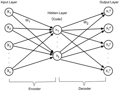
As shown in Fig. 1, the network can be represented as.
(1) Encoding: Input layer + Hidden layer:
Among them, represents the input feature vector, whose dimension is . represents the weight of neurons with a dimension of , where is the number of neurons in the hidden layer and is the number of neurons in the input layer, which is responsible for mapping the input features to the hidden layer. represents the bias of neurons. is the activation function. Commonly used ones include ReLU, Sigmoid or Tanh, etc. The activation function in this paper is Tanh, which is used to introduce nonlinear characteristics. represents the output of the hidden layer, that is, the encoding of the input data, capturing the main features of the input data, with a dimension of .
(2) Decoding: Hidden layer + Output layer:
Among them, represents the weight matrix of the decoder, with a dimension of , which is responsible for mapping the features of the hidden layer back to the original feature space. represents the bias term of the decoder, with a dimension of . represents the ReLU activation function of the decoder. represents the output of the output layer, that is, the reconstructed data, expecting to be as close as possible to the original input data , with a dimension of .
(3) Loss function.
Let represent the weights and bias parameters of the network, then the loss function is:
Among them, represents the loss function of the autoencoder, measuring the difference between the input data and the reconstructed data . represents the weights and bias parameters of the network, including , , and . represents the sample size. represents the input data of the -th sample. represents the reconstructed data of the i-th sample. represents the distance measurement function between the input data and the reconstructed data . Here, the cross-entropy loss is used, and the gradient descent method can be adopted for training. Furthermore, in order to control the degree of weight reduction and prevent overfitting of the autoencoder, a regularization term (also known as the weight decay term) will be added to the above-mentioned loss function to transform it into a regularized autoencoder:
Among them, represents the loss function of the regularized autoencoder. represents the regularization parameter, which is used to control the degree of weight attenuation and prevent overfitting. represents the square of the L2 norm of the weight matrix , which is used for regularization and indirectly makes the neurons in the hidden layer sparse by constraining the network weights, thereby improving the generalization of the entire autoencoder model.
2.2. Convolutional autoencoder (CAE)
Due to the disadvantages of autoencoders such as difficult feature interpretation, sensitivity to data distribution, high demand for training resources, and easy overfitting, while convolutional autoencoders (CAE) retain the spatial information of data through convolutional layers and de-convolutional layers, are suitable for processing high-dimensional data, have low computational complexity, strong feature extraction ability, and good data reconstruction effect. Therefore, convolutional autoencoders are used instead of autoencoders. Convolutional autoencoder is an unsupervised neural network learning algorithm that combines autoencoders and convolutional operations, mainly used for data dimension reduction and feature learning. It consists of two parts: the encoder and the decoder, and its structure is shown in Fig. 2.
Fig. 2CAE model structure diagram
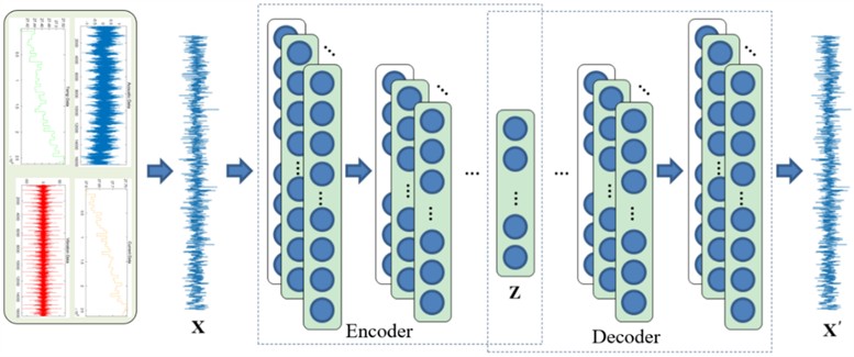
(1) Encoder section.
The encoder part is composed of convolutional layers and pooling layers stacked together. This paper uses one-dimensional convolution operation, and its operation process is as follows:
Among them, * represents the convolution kernel operation, is the output of the -th convolution kernel in the layer, and are the weights and offsets of the -th convolution kernel in the layer, is the output of the JTH convolution kernel in the layer, and is the activation function, such as Sigmoid, ReLU, etc.
The pooling layer reduces the feature size by down-sampling the output of the convolutional layer. The operation formula is as follows:
Among them, is the pooling function, such as maximum pooling, mean pooling, etc., and and are the inputs and outputs of the pooling layer respectively.
(2) Decoder section.
The decoder part of the convolutional autoencoder is composed of stacked transposition convolutional layers, achieving the mapping from low-dimensional features to high-dimensional features. The calculation process of transposed convolution is similar to Eq. (5), and the weights of its convolution kernels are obtained by transposition of the weight in Eq. (5).
2.3. Self-attention mechanism
In order to dynamically allocate weights to different features when extracting features, enabling the model to focus on important feature information more effectively, the self-attention mechanism is invoked. The self-attention mechanism is a variant of the attention mechanism. It reduces the reliance on external information and is better at capturing the internal correlations of data or features. The key point of the self-attention mechanism lies in that , , and are the same thing, or they all originate from the same and have the same origin. Find the key points in through , thereby paying more attention to the key information of and ignoring the unimportant information of . It is not the attention mechanism between the input statement and the output statement, but the attention mechanism that occurs among the internal elements of the input statement or among the internal elements of the output statement.
Fig. 3Self-attention mechanism module structure
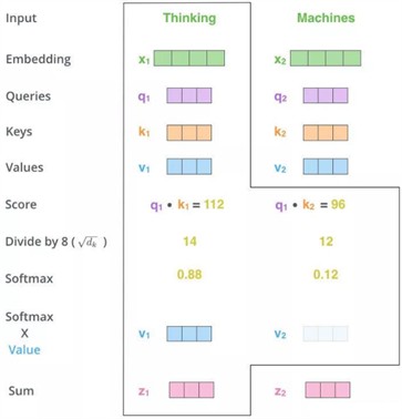
The self-attention module is shown in Fig. 3. First, for each vector , multiply it by three coefficients , , and respectively to obtain , , and , which represent query, key, and value respectively. The three W’s are the parameters which we need to learn. Then, the obtained and are used to calculate the correlation between every two input vectors. Generally, the dot product calculation is adopted, and a score: is calculated for each vector. Then divide the just-obtained similarity by and perform Softmax. After normalization by Softmax, each value is a weight coefficient greater than 0 and less than 1, and the sum is 1. This result can be understood as a weight matrix. Finally, use the just-obtained weight matrix, multiply it by , and calculate the weighted sum.
2.4. Gated autoencoder (GAU)
The time information in the data collected by sensors plays a key role in capturing the operating conditions of machinery [16]. However, a single CNN architecture may not be able to fully explain the temporal dynamics in the data sequence. Since GRU is specifically designed to enhance the interdependence among time series data, the GRU module is referenced to coordinate the time information in the input sequence. Both GRU and LSTM belong to RNN variants [17], which are used to solve the vanishing gradient problem and reflect the emphasis on time information as well as the enhancement of the interdependence among time series data. Compared with the latter, the GRU network has a simpler structure, a faster training speed and higher efficiency. This paper adopts the GRU module, and its structural description is shown in Fig. 4.
Fig. 4The schematic diagram of GRU
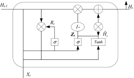
As shown in Fig. 4, GRU combines the forget gate and input gate in the gate mechanism into a single new gate, which is called the update gate. This change has produced a streamlined model with fewer update weights, promoting faster training. The structural formula is expressed as:
Among them, represents the data input, is the implicit state of the input sequence at the previous moment, is the current implicit state of the input sequence, is the candidate implicit state of the input sequence, and represent the two gates of the GRU module, namely the update gate and the reset gate, , , and represent the weight matrices between the two gates and the input layer, , and represent the weight matrices of cyclic connections, and represent the bias terms. and represent activation functions, and represents the dot product.
As shown in Fig. 5, the GAU proposed in this paper mainly includes two stages: encoding the input data features and feature reconstruction after decoding. There is one GRU Encoder layer in the encoding stage, one GRU Decoder layer and one FC fully connected layer in the decoding stage, as well as a global self-attention mechanism.
Fig. 5GAU structure
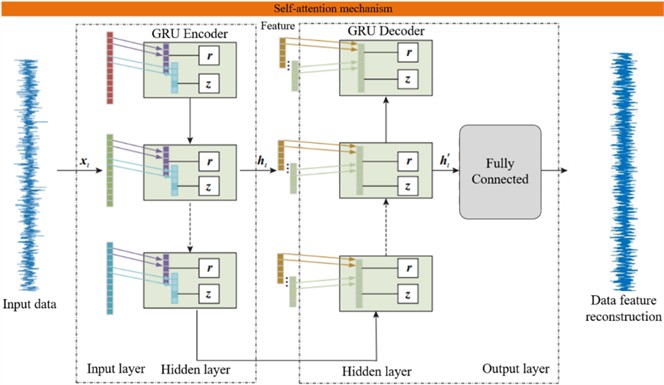
(1) Coding section.
First, the GRU Encoder encodes the features of the input data and extracts the features of the input layer data. The Encoder of GRU is composed of multiple GRU units in a loop. The input of each unit not only includes the input information at the current moment, but also the hidden information of the previous unit, generating a new hidden information . Each GRU unit is composed of update gates, reset gates, etc. The convolution part uses convolution kernels to extract data features, and the calculation formula is:
Among them, and are respectively the loop weights and input weights of each gate at the previous moment.
The update gate can selectively discard some information from the hidden state and decide to add new information to the hidden state. The calculation formula is:
Among them, is the symbol of the sigmoid function. and are the update result and bias parameter of the update gate, respectively.
The reset gate can control the forgetting situation and determine the information that needs to be forgotten. The calculation formula is:
The final output value is determined by Eq. (11) to (13):
Among them, and are the candidate state and the final state respectively.
(2) Decoding part.
The network structure of GRU Decoder is similar to that of the GRU Encoder, except that the encoding operation is replaced by the decoding operation. It contains multiple GRU Decoder units, and the input of each unit includes the output data and the output of the previous unit. Each unit consists of a decoding part, an update gate, a reset gate, etc. The decoding part checks the input and extracts features. The calculation formula is:
Among them, and are respectively the loop weights and input weights of each gate at the previous moment.
3. Flowchart of diagnosis method based on the proposed model
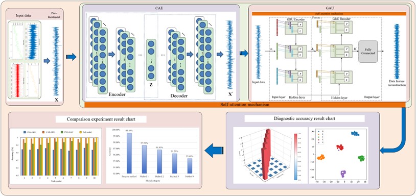
The diagnostic flowchart of this paper is shown in Fig. 6. Firstly, the input multi-source data set is preprocessed, including steps such as data cleaning, transformation, standardization and normalization, to fuse the multi-source data set into a new data. The spatial features of this data are extracted by CAE, and the input data is compressed into a low-dimensional hidden representation through the convolutional layer and pooling layer to reduce the complexity of data. Then, the GRU_Encoder is used to model the time series data and capture the time dependency, and the GRU_Decoder is used to decode the encoded features and reconstruct the features to achieve sequence modeling and feature reconstruction. At this point, GAU uses the gating mechanism to further process the hidden representation, highlighting important features and suppressing unimportant ones. During this process, the self-attention mechanism can not only dynamically allocate weights to different features, enabling the model to focus on important feature information more effectively, but also perform weighted fusion on the extracted features through the self-attention mechanism. Finally, the softmax classifier is used to achieve fault classification. According to the optimized model parameters, the fault diagnosis results are output, and the model is evaluated and verified using evaluation indicators such as accuracy rate, loss rate, and confusion matrix.
Fig. 6Diagnostic flowchart
4. Experiment verification and comparison study
4.1. NSK 6205 DDU dataset
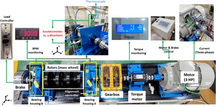
The standardized NSK bearing (NSK 6205 DDU) dataset [18] is provided by the Korea Mechanical Research Institute. The test bench shown in Fig. 7 is a rotating mechanical testing system, including a three-phase induction motor, torque sensor, gearbox, two bearing seats (A and B), rotor, and hysteresis brake. The maximum speed of the motor is 3663 RPM, and the test runs at 3010 RPM to avoid interference. The torque is applied by the hysteresis brake, and the load is measured by a torque meter, which is divided into three levels: 0, 2, and 4 N·m. Acoustic data is collected under no-load conditions to reduce the impact of hysteresis brake air cooling noise on the microphone.
Fig. 7Rotating machine data set test bench
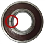
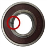
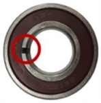
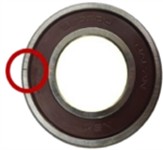
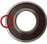
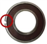
When conducting tests under variable load conditions, different sizes of cracks as shown in Fig. 8 are set to simulate bearing damage, which occurs on the inner or outer ring.
Fig. 8Bearing by crack size: a) inner race 0.3 mm, b) inner race 1.0 mm, c) inner race 3.0 mm, d) outer race 0.3 mm, e) outer race 1.0 mm, and f) outer race 3.0 mm
a)
b)
c)
d)
e)
f)
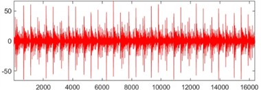
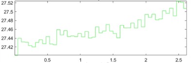
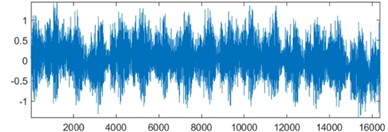
Carry out the test at 3010 RPM with applied brake load torques of 0, 2, and 4 N·m. Acoustic data is collected under no-load conditions to reduce noise interference. The variable load test aims to simulate bearing damage, including cracks in the inner and outer rings. The used heterogeneous data covers five types of faults, including vibration, acoustic, and current data of healthy bearings under 0 N·m load, temperature data under 2 N·m load, data on inner and outer ring faults (0.3 mm and 1.0 mm) under 0 N·m load, and temperature data under 2 Nm load. The time domain diagram collected signals are shown in Fig. 9.
In this study, standardization and sliding window methods are used to preprocess the network input data. Due to the large amount of single fault data, a window length of 4096 data points and a step size of 64 are used to create training data, which is randomly divided into datasets for training and testing. The details of multi-source sample division are shown in Table 1. Among them, the sliding window method is mainly used to extract multiple overlapping samples from the input sequence (as shown in Fig. 10).
Fig. 9The time-domain waveforms of four types of sensor data: a) vibration data; b) temperature data; c) acoustic data; d) current data
a)
b)
c)
d)
Table 1Division table of training and test data
Data type | Fault type | Loads | Total samples | Partitioning ratio of training set | Partitioning ratio of test set |
Temperature | Healthy bearing | 2 Nm | 200000 | 70 % | 30 % |
Inner race fault (0.3 mm) | |||||
Inner race fault (1.0 mm) | |||||
Outer race fault (0.3 mm) | |||||
Inner race fault (0.3 mm) | |||||
Acoustic | Healthy bearing | 0 Nm | 200000 | 70 % | 30 % |
Inner race fault (0.3 mm) | |||||
Inner race fault (1.0 mm) | |||||
Outer race fault (0.3 mm) | |||||
Inner race fault (1.0 mm) | |||||
Vibration | Healthy bearing | 0 Nm | 200000 | 70 % | 30 % |
Inner race fault (0.3 mm) | |||||
Inner race fault (1.0 mm) | |||||
Outer race fault (0.3 mm) | |||||
Inner race fault (1.0 mm) | |||||
Current | Healthy bearing | 0 Nm | 200000 | 70 % | 30 % |
Inner race fault (0.3 mm) | |||||
Inner race fault (1.0 mm) | |||||
Outer race fault (0.3 mm) | |||||
Inner race fault (1.0 mm) |
4.2. Results and analysis
The key parameters used in the proposed CAE-GAU model and the corresponding reasons are shown in Table 2.
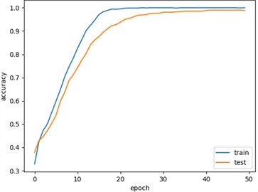
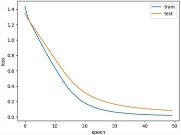
Fig. 11 shows the training and testing curves for the standardized NSK bearing (NSK 6205 DDU) dataset, with an accuracy curve of 98.78 % as shown in Fig. 11(a) and a loss rate curve of 8.3 % as shown in Fig. 11(b).
Fig. 10Sliding window data augmentation
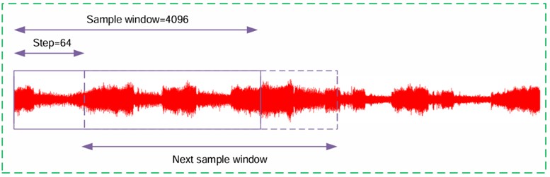
Table 2Key parameters of the proposed model
Parameters | Meanings | Value | Reasons |
Number of convolutional layers | The number of convolutional layers used to extract spatial features from data in CAE | 3 | Based on experience and experimental results, it has been determined that within a certain range of convolutional layers, features can be effectively extracted while avoiding overfitting |
Number of convolution kernels | The number of convolution kernels in each convolutional layer | 16, 32, 64 | The gradually increasing number of convolution kernels can extract richer features layer by layer, making it suitable for processing complex data features |
Size of convolutional kernel | The spatial size of convolutional kernels | 3×3 | While maintaining a certain receptive field, it can capture local features well and has moderate computational complexity |
Type and size of pooling layer | Types of pooling operations and pooling window sizes used for down-sampling | Maxim-um pooling, 2×2 | Maximum pooling can preserve the main information of features to a certain extent, and a 2×2 pooling window size reduces the feature dimension without losing too much information |
Number of GRU units | The number of units in GRU encoder and decoder in GAU | 128 | After multiple experimental verifications, the number of units can achieve a good balance between model performance and computational complexity |
GRU layers | The number of layers of GRU encoder and decoder in GAU | 2 | The two-layer GRU structure can capture longer temporal dependencies in time series while avoiding gradient vanishing and excessive computational burden caused by too many layers |
Number of fully connected layer neurons | The number of fully connected layer neurons used for feature fusion and classification in the final model | 128 | This quantity can effectively fuse and transform the extracted features, providing appropriate feature representations for the classifier |
Learning ratio | Step size for updating model parameters during optimization process | 0.001 | A smaller learning rate can ensure stable convergence of the model during training, and after adjusting the learning rate decay strategy, it can also better adapt to the needs of different training stages |
Batch size | The number of samples used to update model parameters in each training iteration | 64 | This batch size can ensure the stability of model training while fully utilizing the parallel computing power of GPU to improve training efficiency |
Training rounds | The number of times the model is trained on the entire training dataset | 100 | After a certain number of training rounds, the model can fully learn data features and converge on the training set. Excessive training rounds may lead to overfitting, while 100 rounds perform well in ensuring model performance and preventing overfitting |
Regularization parameter | Regularization term coefficients used to prevent model overfitting | 0.0001 | Smaller regularization parameters can moderately constrain the parameters while preserving the model's learning ability, reducing the model's sensitivity to noise and overfitting |
Activation function type | The activation functions used in each layer of the model | ReLU, Tanh | The ReLU activation function can introduce nonlinearity and has high computational efficiency, making it suitable for use in convolutional layers; The Tanh activation function in GRU units can limit the output values within a certain range, which helps stabilize the training process of the model |
Type of optimizer | Optimization algorithm for updating model parameters | Adam | The Adam optimizer combines the advantages of momentum and RMSprop, which can adaptively adjust the learning rate, accelerate the training process of the model, and improve the convergence effect |
Fig. 11Training and testing curves: a) precision curve; b) loss rate curve
a)
b)
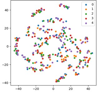
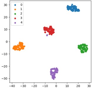
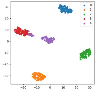
Fig. 12 shows the t-SNE feature visualization results of the standardized NSK bearing (NSK 6205 DDU) dataset by using the proposed method, which can clearly and intuitively reflect the model's processing effect on features and the separability of features at different levels. This is of great significance for understanding the internal working mechanism of the model and evaluating its performance. The visualization of the input features to the first layer shown in Fig. 12(a) shows a relatively scattered distribution of feature points, with various types of data mixed together without forming clear clusters or boundaries, and only 67.15 % classification accuracy is obtained. This phenomenon fully indicates that the separability of the original features in the initial stage is poor and cannot be directly used for effective classification tasks. It also implies the necessity of deep processing and extraction of the original features. In Fig. 12(b), the visualization results of the features output in the last layer present a completely different scene, and 98.78 % classification accuracy is obtained. After fine processing by the CAE-GAU model, the feature distribution has undergone significant changes, with various feature points clustered tightly and forming clear boundaries. This clearly demonstrates the powerful feature extraction and transformation capabilities of the CAE-GAU model. Specifically, the model encodes and decodes the original features through a convolutional autoencoder to extract more representative spatial features. Then, the self attention mechanism focuses on key features, dynamically adjusts feature weights, and further enhances feature discriminability. Finally, the gate controlled autoencoder effectively controls the flow of information during the feature conversion process, ensuring a steady improvement in feature quality. This enables the model to learn high-quality and more discriminative feature representations, laying a solid foundation for subsequent classification tasks and greatly improving the success rate and accuracy of classification tasks.
Fig. 12Visualization of t-SNE features: a) visualization of the features input to the first layer; b) visualization of the features output at the last layer
a)
b)
In terms of model diagnosis and performance evaluation, we have recorded the following key indicators to comprehensively reflect the efficiency and performance of the model. The computer configuration used in the experiment is: Intel Core AMD RyzenTM9-5900HX processor, with a clock speed of 3.3 GHz, equipped with NVIDIA GeForce RTX 3080 graphics card (16GB of video memory), the system is equipped with 32 GB of memory, runs Windows 11 Home Edition, and is equipped with solid-state memory, with a total capacity of about 2TB. In this hardware environment, the total training time of CAE-GAU model is about 23 minutes, including about 3.4 minutes for data preprocessing stage, about 15.5 minutes for model training stage, and about 4.1 minutes for testing stage. In addition, during the model training process, the average computation time for a single iteration is 30 seconds, and the model converges quickly on the training set. After about 20 epochs, the loss function tends to stabilize, indicating that the model has good convergence performance. The parameter count of the model is 800000, with a memory usage of approximately 4.6 GB during training and 3.2 GB during testing. The overall resource consumption is within an acceptable range and has good efficiency performance, which can meet the requirements for model running efficiency in practical industrial scenarios.
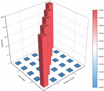
The 3D confusion matrix is an intuitive tool for evaluating the classification performance of a model. The values on the diagonal of the matrix represent the number of correctly classified samples, while the values on the non diagonal represent the number of misclassified samples. Compared to two-dimensional confusion matrices, three-dimensional confusion matrices can more intuitively and comprehensively display the confusion between categories in multi classification problems. It adds a dimension to clearly present the degree of confusion between each category and all other categories, avoiding the problem of information overlap or difficulty in distinguishing in the two-dimensional plane, which helps to more accurately evaluate the model's ability to identify different types of faults. Meanwhile, the geometric structure in three-dimensional space can better display classification boundaries and misclassification patterns, enabling us to quickly locate weak links in the model and optimize them accordingly. In addition, the three-dimensional confusion matrix can better maintain the clarity of the visualization effect compared to the two-dimensional matrix when displaying complex relationships of multiple categories, which is more in line with the complexity of multi classification problems and provides stronger support for model performance evaluation. The three-dimensional confusion matrix for the standardized NSK bearing (NSK 6205 DDU) dataset using the proposed method is presented in Fig. 13. It can be intuitively observed from the figure that the elements on the diagonal occupy an absolute dominant position, with significantly higher values than non diagonal elements. Among them, the probability of correctly classifying healthy samples is 100.00 %, and among the samples with inner circle faults of 0.3mm, 98.78 % are correctly classified and 1.22 % are incorrectly classified as inner circle faults of 1.0mm. These data indicate that the model has significant classification advantages on the NSK 6205 DDU dataset and can achieve high accuracy in fault diagnosis. This strongly indicates that the model has excellent accuracy in most categories and can accurately distinguish data from different categories, fully reflecting its outstanding performance in handling multi classification problems. Further analysis of the misclassification situation of each category reveals that although there may be individual sample confusion in a few categories, the overall trend shows that the model exhibits strong generalization ability and recognition ability for complex data patterns. For example, on some samples with similar features or near the decision boundary, the model can still control the misclassification rate at a low level with its strong feature expression ability. This not only verifies the effectiveness of the CAE-GAU model in this task, but also reflects the adaptability and robustness of the model to complex data distributions in practical applications, enabling it to stably and reliably complete classification tasks in the face of diverse and complex real-world scenarios, providing strong support for practical applications in related fields.
Fig. 13The three-dimensional confusion matrix of the method proposed in this paper
4.3. Comparison study
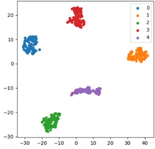
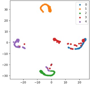
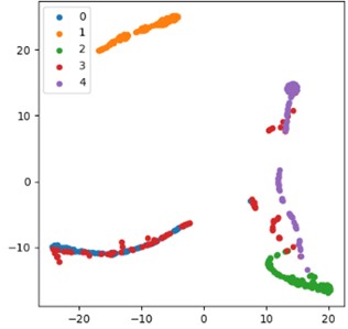
Fig. 14 provides a visual comparison of the t-SNE characteristics of the ablation experimental models. By comparing the feature distribution of different models, we can deeply analyze the key roles of each component in model performance and the differences in the impact of different model combinations on feature expression ability. The feature distribution of the complete CAE-GAU model in Fig. 14(a) shows a highly clustered and highly separated state of various features, thanks to the synergistic effect of the components in the model. Convolutional autoencoder plays a crucial role in the early stage of feature extraction, as it can accurately capture local features in the original data and effectively compress and reconstruct the features through encoding and decoding processes, providing a high-quality feature foundation for subsequent processing. The self attention mechanism plays a core role in the feature optimization process, dynamically adjusting the weights of feature channels or spatial dimensions, highlighting key feature information, suppressing irrelevant noise interference, making features more discriminative and targeted, thereby improving the model’s ability to distinguish between different categories of features. Gated autoencoders use gating mechanisms to reasonably control the flow and updating of information during feature transformation, ensuring that important information being retained while redundant components are removed, further optimizing feature quality, and achieving the best state of feature extraction, transformation, and expression for the complete model, providing the strongest support for classification tasks with 98.78 % classification accuracy being obtained.
Fig. 14Visual comparison of t-SNE characteristics of the ablation experimental model: a) full model; b) CAE-GRU; c) CNN-GAU; d) CNN-GRU
a) Full model
b) CAE-GRU
c) CNN-GAU
d) CNN-GRU
Fig. 14(b) shows the feature distribution of the CAE-GRU model: Although the convolutional autoencoder can extract certain features, the lack of self attention mechanism significantly reduces the focus and discrimination of the features. The lack of self attention mechanism leads to the inability of the model to effectively capture global dependencies and key feature information between features. When dealing with complex feature relationships and multi class discrimination tasks, the feature expression ability is limited, and it cannot accurately focus on key features and suppress noise interference like the proposed model, resulting in loose feature distribution, unclear boundaries between categories, and reduced classification accuracy with 93.47 % classification accuracy being obtained. This phenomenon fully demonstrates the indispensable role of self attention mechanism in feature optimization and improving model performance. By dynamically adjusting feature weights, the discriminative and expressive ability of features can be significantly enhanced, thereby improving the model's ability to distinguish between different categories of features.
Fig. 14(c) shows the feature distribution of the CNN-GAU model, which only uses the combination of convolution and gated autoencoder, and the compactness and separability of the features are not as good as the proposed model. Although convolutional layers can extract local features, there is a lack of deep encoding and decoding processing of features by convolutional autoencoders in the early stage of feature extraction, which cannot fully explore the inherent structure and hierarchical information of features, resulting in insufficient and refined feature expression. Although the gated autoencoder plays a certain role in the feature transformation process, the subsequent feature transformation and optimization are also difficult to achieve the desired effect due to the insufficient quality of the initial features, ultimately limiting the compactness and separability of the feature distribution. The model’s performance in classification tasks cannot be compared to the complete model with 87.32 % classification accuracy being obtained. This comparison highlights the crucial role of convolutional autoencoders in the early stages of feature extraction. By deeply encoding and decoding the original features, they can effectively extract more representative and hierarchical features, providing a solid foundation for subsequent feature transformation and classification tasks.
Fig. 14(d) shows the feature distribution of the CNN-GRU model, which has a relatively loose clustering effect, indicating that the combination of convolution and gated recurrent units has significant shortcomings in feature processing. When the local features extracted by the convolutional layer are processed by the gated loop unit, the quality and expressive ability of the features are greatly affected due to the lack of optimization of self attention mechanism and deep processing of convolutional autoencoder. Although the gated recurrent unit can process sequence information, if there is a lack of effective capture of global dependencies of features and deep mining of feature levels when combined with convolution, the feature distribution will be difficult to form a compact and clear clustering structure, resulting in poor feature separability and greatly reduced performance of the model in classification tasks with 81.65 % classification accuracy being obtained. This phenomenon further proves the necessity of the collaborative effect of various components in the CAE-GAU model to improve feature quality. The lack of any key component may lead to a decrease in feature expression ability, thereby affecting the overall performance of the model.
Fig. 15Comparison of the results of 10 ablation experiments
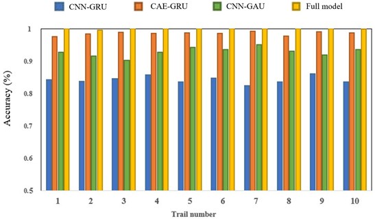
Fig. 15 shows the comparison results of 10 ablation experiments. It can be clearly seen from the figure that the proposed method achieves the most outstanding and stable results in terms of performance. Specifically, the proposed method achieves a diagnostic accuracy of 99.49 %, which is 4.61 % higher than the CAE-GRU model. Compared to the CNN-GAU model, it has improved by 8.71 %. Compared to the CNN-GRU model, it has improved by 14.46 %. The performance indicators of the complete CAE-GAU model have been superior to other variant models in multiple experiments, indicating that the combination of self attention mechanism and convolutional autoencoder is complementary and can fully leverage the advantages of the model in feature extraction, feature transformation, and classification prediction. By comparison, the CAE-GRU model performs poorly in handling complex feature relationships due to the lack of self attention mechanism, especially in reducing accuracy in multi class discrimination. Although the CNN-GAU model introduces gated autoencoders, it lacks the efficient feature extraction capability of convolutional autoencoders, resulting in insufficient feature expression. The CNN-GRU model has the weakest feature processing ability and the lowest classification accuracy due to the lack of self attention mechanism and optimization of convolutional autoencoder. This comparative result further validates the rationality and superiority of the overall architecture of the CAE-GAU model, indicating that each component cooperates and synergizes in the complete model, which has a significant effect on improving the performance of the model in related tasks. From the stability analysis of the experimental results, the proposed model shows minimal performance fluctuations in multiple experiments, demonstrating strong stability, while other models exhibited varying degrees of performance fluctuations in different experiments, further highlighting the reliability of the complete model.
Table 3 shows the mean and variance of the ten ablation experimental models, and it can be seen that the complete model in this article has a mean of 0.98 and a variance of 0.003, indicating stable performance and high accuracy. CAE-GRU lacks self attention mechanism, resulting in decreased performance with a mean of 0.91 and variance of 0.005, indicating slight fluctuations in performance. CNN-GAU lacks a convolutional autoencoder, resulting in further performance degradation with a mean of 0.87 and variance of 0.009, indicating significant fluctuations. CNN-GRU lacks self attention mechanism and convolutional autoencoder, with the worst performance, a mean of 0.83, variance of 0.012, and the largest fluctuation.
Table 3Table of mean and variance in ablation experiments
Model | Mean | Variance |
CNN-GRU | 0.83 | 0.012 |
CNN-GAU | 0.87 | 0.009 |
CAE-GRU | 0.91 | 0.005 |
Full model | 0.98 | 0.003 |
From the stability analysis of the experimental results, the proposed model shows minimal performance fluctuations in 10 experiments, demonstrating exceptional stability. This is mainly due to the reasonable architecture and collaborative working mechanism of each component in the model. The self attention mechanism, convolutional autoencoder, and gated autoencoder work together to construct a stable and efficient feature processing flow, which enables the model to maintain stable and excellent performance under different experimental conditions. However, other models exhibit varying degrees of performance fluctuations in different experiments. For example, the CAE-GRU model may experience significant performance degradation in certain experiments due to changes in data distribution or increased feature complexity, while the CNN-GAU and CNN-GRU models also have similar issues, further highlighting the reliability of the complete model. Overall, the CAE-GAU model demonstrates outstanding performance in feature extraction, transformation, classification, and model stability due to its complete architecture and synergistic effects of various components. It provides the most reliable solution for related tasks and has broad application prospects and practical value.
The proposed method will be compared and analyzed with current advanced multi-source dataset fault diagnosis methods, involving the following latest models:
1) DAMFR-LSTM model: DAMFR-LSTM is a deep feature extraction and predictive fault diagnosis method that integrates multi-source information. Its focus is on the feature extraction stage, using DAMFR technology to extract the feature subset with the largest amount of information, avoiding the problem of improper feature extraction in traditional LSTM networks, and thus improving the accuracy of fault diagnosis. DAMFR-LSTM utilizes the LSTM model to construct a deep neural network feature learning tool for fault diagnosis, which has higher accuracy compared to other feature extraction methods.
2) Method based on multi-source monitoring data fusion: This method divides and processes multi-source monitoring data through different time window lengths, and stores them in different datasets to obtain corresponding multi-source monitoring datasets. Then extract features from each dataset separately to obtain multi-source feature data. Finally, the multi-source feature data corresponding to each time window length is fused to obtain multi time window fusion data for fault diagnosis. This method can better extract feature data that characterizes equipment failure modes.
3) Fault diagnosis method for multi-source time-series data based on graph neural network: Preprocess multi-source time-series historical data to obtain training samples, including steps such as data synchronization, normalization, and data slicing. Then, by training the graph neural network model with training samples, a fault diagnosis model is obtained. For the system to be tested, obtain real-time data from multiple sources and preprocess it before inputting it into the fault diagnosis model, and output the fault diagnosis results of the system. This method can integrate the correlation features of multi-source data and the temporal characteristics of the time dimension, improving the accuracy and noise resistance of fault diagnosis.
4) A multi-source sensor fault diagnosis method based on an improved CNN-GRU network: This method combines multi-source sensor data with unified sampling frequency and time alignment, concatenates them into a two-dimensional matrix, and slices it. CNN is used to extract spatial features to obtain feature maps, and GRU is used to extract temporal features of the feature maps, ultimately obtaining fault information. Add a sensor data calibration module to the convolutional network and a fault category parsing module to the recurrent network to extract intermediate layer features, calculate fault category information, and pass it to the parameter estimation network.
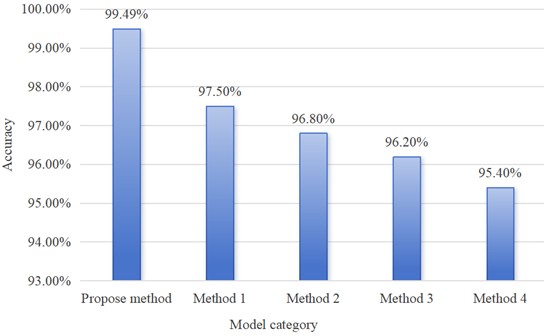
The experimental results are shown in Fig. 16, and the proposed method achieved a satisfactory diagnostic accuracy of 99.49 %, demonstrating excellent performance. In contrast, the diagnostic accuracy of the DAMFR-LSTM model is 97.50 %. The diagnostic accuracy of the method based on multi-source monitoring data fusion is 96.80 %, which is 2.69 % lower than the proposed method. The diagnostic accuracy of the multi-source time-series data fault diagnosis method based on graph neural network is 96.20 %, which is 3.29 % lower than the proposed method. The diagnostic accuracy of the multi-source sensor fault diagnosis method based on the improved CNN-GRU network is 95.40 %, which is 4.09 % lower than the proposed method. This difference demonstrates that the proposed method can more effectively extract and utilize features from multi-source datasets, providing higher diagnostic accuracy.
Fig. 16Comparative analysis among advanced models. Method 1: DAMFR-LSTM model; Method 2: Method based on Multi-source monitoring data fusion; Method 3: Multi-source Time series data fault diagnosis method based on Graph neural network; Method 4: Multi-source sensor fault diagnosis method based on Improved CNN-GRU network
In order to demonstrate the advantages of the method compared to the comparative method in Fig. 16 from multiple perspectives, Table 4 presents score statistics from multiple dimensions such as time efficiency and F1 score.
Table 4Comparison table of performance evaluation parameters
Method | Training times | Single-sample inference speed | F1-score | Recall |
Propose method | 23 mins | 0.011 ms | 98.38 % | 94 % |
Method 1 | 59 mins | 2.142 ms | 96.4 % | 92 % |
Method 2 | 1 h 2 mins | 4.54 ms | 95.7 % | 90 % |
Method 3 | 1 h 12 mins | 10.318 ms | 94.2 % | 88 % |
Method 4 | 51 mins | 0.233 ms | 92.9 % | 87 % |
5. Conclusions
In summary, this article proposes an innovative diagnostic method based on CAE-GAU (a combination of convolutional autoencoder and gated autoencoder) for fault diagnosis of complex multi-source heterogeneous data. This method combines the advantages of Convolutional Autoencoder (CAE) and Gated Autoencoder Unit (GAU), and introduces self attention mechanism to effectively solve the problems of difficult feature extraction and insufficient diagnostic accuracy in traditional fault diagnosis methods when dealing with multi-source heterogeneous data.
In the feature extraction stage, CAE can accurately capture local features in the raw data and compress the input data into low dimensional hidden representations through convolutional and pooling layers, reducing data complexity while preserving key information. Subsequently, GAU utilizes gating mechanisms to further process hidden representations, highlighting important features and suppressing unimportant ones, enhancing the model's ability to reconstruct features. The self-attention mechanism dynamically adjusts the weights of feature channels or spatial dimensions, highlights key feature information, suppresses irrelevant noise interference, and makes features more discriminative and targeted, thereby improving the model's ability to distinguish between different categories of features.
The experiment uses the NSK 6205 DDU dataset, which covers multiple types of faults and different load conditions, and has high complexity and representativeness. The effectiveness and superiority of the proposed method were fully verified through ablation experiments and comparative experiments. In the ablation experiment, the complete CAE-GAU model showed the best and most stable performance in multiple experiments, achieving a diagnostic accuracy of 99.49 %, an improvement of 4.61 % compared to the CAE-GRU model, an improvement of 8.71 % compared to the CNN-GAU model, and an improvement of 14.46 % compared to the CNN-GRU model. The experimental results show that the components work together and synergistically in the complete model, which has a significant effect on improving the performance of the model in related tasks.
Compared with other advanced fault diagnosis methods, such as DAMFR-LSTM model, method based on multi-source monitoring data fusion, multi-source time-series data fault diagnosis method based on graph neural network, and multi-source sensor fault diagnosis method based on improved CNN-GRU network, the method proposed in this paper achieved accuracy improvements of 1.99 %, 2.69 %, 3.29 %, and 4.09 %, respectively. This difference demonstrates that the proposed method can more effectively extract and utilize features from multi-source datasets, providing higher diagnostic accuracy.
The experimental results show that the proposed method exhibits excellent performance and reliability in handling fault diagnosis problems under multi-source heterogeneous data conditions. Specifically, this method can effectively handle multi-source data fusion problems, complex data distribution problems, multi class fault recognition problems, and scenarios with high real-time requirements.
In future research, with the continuous development of industrial Internet of Things and big data technology, multi-source heterogeneous data fault diagnosis methods will play a key role in a wider range of industrial scenarios. The method proposed in this article not only provides a new technical idea for the field of fault diagnosis, but also provides valuable reference for related research, which is expected to promote the development of fault diagnosis technology towards higher accuracy, stronger adaptability, and wider application areas.
References
-
J. Sun et al., “The variable condition of rolling bearing fault diagnosis based on improved CNN,” Journal of Thermal Power Engineering, Vol. 40, No. 2, pp. 176–186, Feb. 2025.
-
S. Li et al., “Based on fractional order of Adam GRU helped bearing fault diagnosis of neural network,” Automation and Instrument, Vol. 40, No. 4, p. 60, Mar. 2025, https://doi.org/10.19557/j.cnki.1001-9944.2025.04.011
-
B. Zhang et al., “Transformer discharge fault diagnosis method based on synchronous compressed wavelet transform and ResNet,” The Modern Electronic Technology, Vol. 46, No. 10, pp. 159–165, May 2023, https://doi.org/10.16652/j.issn.1004-373x.2023.10.030
-
J. P. Tang et al., “Fault diagnosis method of gas turbine rotor based on WDCNN-SVM deep transfer learning,” Journal of Electronic Measurement and Instrument, Vol. 35, No. 11, pp. 115–123, Nov. 2021, https://doi.org/10.13382/j.jemi.b2003813
-
F. Yan, C. J. Xiao, and Y. W. Sun, “Rolling bearing fault diagnosis based on SVD and 1DCNN,” Journal of Civil Aviation Flight University of China, Vol. 35, No. 5, pp. 37–42, Sep. 2024.
-
J. Yang, J. Chen, X. Zhan, C. Liu, and C. Yang, “A feature reconstruction and SAE model based diagnosis method for multiple mixed faults,” Measurement Science and Technology, Vol. 35, No. 8, p. 086130, Aug. 2024, https://doi.org/10.1088/1361-6501/ad4c8b
-
Y. Li, J. Li, and S. Chen, “A new multi-domain entropy signal classification method,” Applied Acoustics, Vol. 231, p. 110521, Mar. 2025, https://doi.org/10.1016/j.apacoust.2024.110521
-
C. Y. Lu et al., “Two-stage adversarial transfer fault diagnosis method based on dual feature extractors under strong noise interference,” Coal mine machinery, Vol. 46-48, No. 5, pp. 167–170, Apr. 2025, https://doi.org/10.13436/j.mkjx.202505046
-
G. J. Cai, “Bearing fault diagnosis method based on multi-scale convolutional autoencoder,” China Equipment Engineering, Vol. 7, pp. 173–177, Mar. 2025.
-
Q. Z. Yang and P. Wang, “Of Marine diesel engine fault diagnosis based on the encoder research,” Mechanical management and development, Vol. 40, No. 3, pp. 63–65, Oct. 2024, https://doi.org/10.16525/j.cnki.cn14-1134/th.2025.03.022
-
Z. Y. Yin, S. Y. Liu, and F. Q. Zhang, “Fault diagnosis method for aero-engine bearings based on CAE-LSTM,” Journal of Chinese Computer Systems, Vol. 21, No. 1, pp. 5–9, Jul. 2025, https://doi.org/10.19665/j.issn1001-2400.2022.06.017
-
H. W. Zheng, K. Wang, and Y. Cheng, “Bearing fault diagnosis method based on parallel feature extraction,” Noise and Vibration Control, Vol. 44, No. 6, pp. 185–190, Dec. 2024, https://doi.org/10.1006-1355(2024)06-0185-06+197
-
R. Liu, F. Wang, B. Yang, and S. J. Qin, “Multiscale kernel based residual convolutional neural network for motor fault diagnosis under nonstationary conditions,” IEEE Transactions on Industrial Informatics, Vol. 16, No. 6, pp. 3797–3806, Jun. 2020, https://doi.org/10.1109/tii.2019.2941868
-
Y. Long, W. Zhou, and Y. Luo, “A fault diagnosis method based on one-dimensional data enhancement and convolutional neural network,” Measurement, Vol. 180, p. 109532, Aug. 2021, https://doi.org/10.1016/j.measurement.2021.109532
-
Y. Yu, H. R. Karimi, L. Gelman, and A. E. Cetin, “MSIFT: A novel end-to-end mechanical fault diagnosis framework under limited and imbalanced data using multi-source information fusion,” Expert Systems with Applications, Vol. 274, p. 126947, May 2025, https://doi.org/10.1016/j.eswa.2025.126947
-
R. Zhao, D. Wang, R. Yan, K. Mao, F. Shen, and J. Wang, “Machine health monitoring using local feature-based gated recurrent unit networks,” IEEE Transactions on Industrial Electronics, Vol. 65, No. 2, pp. 1539–1548, Feb. 2018, https://doi.org/10.1109/tie.2017.2733438
-
J. W. Shi and L. Q. Hou, “Bearing fault diagnosis based on 1D CNN attention gated recurrent network and transfer learning,” Journal of vibration and shock, Vol. 42, No. 3, pp. 159–164, Feb. 2023, https://doi.org/10.13465/j.cnki.jvs.2023.03.018
-
W. Jung, S.-H. Kim, S.-H. Yun, J. Bae, and Y.-H. Park, “Vibration, acoustic, temperature, and motor current dataset of rotating machine under varying operating conditions for fault diagnosis,” Data in Brief, Vol. 48, p. 109049, Jun. 2023, https://doi.org/10.1016/j.dib.2023.109049
About this article

The paper is supported by Henan Province’s New Key Discipline – Machinery (Grant No. 0203240011).
The datasets generated during and/or analyzed during the current study are available from the corresponding author on reasonable request.
Shuai Zheng: concept and writing of the entire paper. Zhiguo Ma: algorithm, implementation.
The authors declare that they have no conflict of interest.
