Abstract
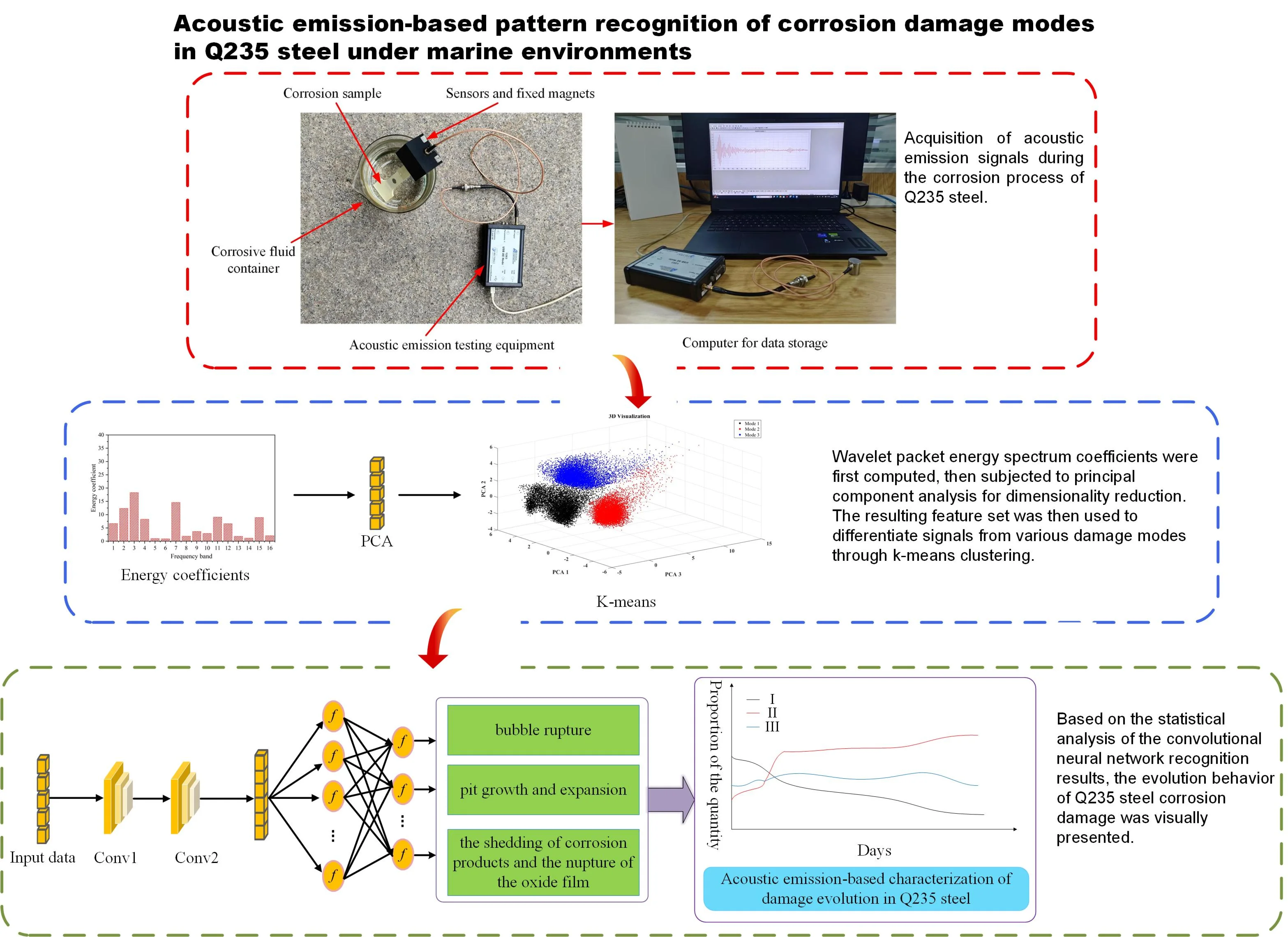
To overcome the limitations of traditional monitoring methods, which are restricted to periodic inspections, this study proposes a real-time method for identifying metal corrosion damage patterns to monitor the condition of Q235 steel corrosion based on acoustic emission (AE). Firstly, AE technology was utilized to monitor the corrosion process of Q235 steel plates in simulated industrial marine environment in real-time. Wavelet packet energy spectrum coefficients, closely related to the damage mechanism, were extracted from the acquired signals. A feature matrix was then constructed using principal component analysis (PCA) to eliminate redundant information and enhance computational efficiency. The K-means clustering algorithm was then applied to classify the AE signals into three classifications: the signals of mode 1 correspond to bubble rupture, the signals of mode 2 to pit growth and expansion, and the signals of mode 3 to the detachment of corrosion products and oxide film rupture. A damage pattern recognition model based on a convolutional neural network (CNN) was developed, enabling the real-time recognition of other unknown AE signals generating during the corrosion process of Q235 steel, and it exhibited satisfactory performance in accurately identifying corrosion-related acoustic emission patterns.
Highlights
- Wavelet packet decomposition combined with PCA enables effective feature extraction and dimensionality reduction.
- Establishing correlations between acoustic emission signals and microscopic damage enhances Q235 steel corrosion monitoring understanding.
- The CNN-based model enabled reliable recognition and real-time monitoring of signals from Q235 steel corrosion.
1. Introduction
Q235 steel has been significantly developed and widely used in marine engineering and coastal infrastructure due to its excellent strength and durability [1, 2]. However, prolonged exposure to harsh environments with high salinity and humidity presents significant corrosion challenges for Q235 steel [3]. Corrosion not only degrades material properties and damages structures but also heightens the risk of safety incidents [4]. Exploring a reliable monitoring technology and corrosion damage assessment method is crucial for ensuring the long-term safety of steel structures in marine environments. Acoustic emission, as a mature nondestructive testing technology, provides real-time and dynamic monitoring capabilities, offering distinct advantages over traditional methods such as ultrasonic testing, magnetic particle testing, and eddy current testing, while exerting minimal impact on the structure [5, 6]. This technique has been widely applied in various fields, including aerospace, machinery manufacturing, petrochemicals, construction engineering, and materials testing [7-10].
Corrosion-induced growth of internal pits and propagation of microcracks are the primary mechanisms underlying steel failure. As an irreversible energy dissipation process, it releases strain energy from the material in the form of transient elastic waves, referred to as acoustic emission [11]. Acoustic emission signals arise from microscopic defects within the material, with each signal encoding information about the dynamic evolution of these defects [12]. Therefore, by analyzing the acoustic emission signals containing information about microscopic defects, the dynamic evolution of material corrosion damage can be understood, thereby enabling the discrimination of damage patterns. This approach is crucial for advancing studies on the corrosion behavior of Q235 steel in marine environments.
The basic parameter analysis method of AE is the simplest and most straightforward approach to analyze material damage characteristics. Although the AE parameter analysis method can qualitatively characterize material damage properties [13-15], it has significant limitations in identifying micro-damage mechanisms [16]. In contrast, transient signal analysis excels in characterizing micro-damage mechanisms. AE signals are transient and random, containing diverse frequency components and pattern features. Research indicates that acoustic emission signals from different damage modes exhibit distinct frequency characteristics [17, 18]. Wavelet packet transform (WPT) known for its strong time-frequency localization and decomposition capabilities, enables feature extraction across various time and frequency domains. This method provides a robust foundation for extracting acoustic emission signal features and identifying different types of damage [19-21].
Artificial neural networks, known for their nonlinear mapping, adaptive learning, and noise resistance, can automatically extract features from AE signals, enabling accurate identification of different damage modes. Zhao et al. [22] applied continuous wavelet transform to convert the AE signals into input images, then extracted features from the images with CNN, enabling the automatic localization of damaged regions. Cui et al. [23] successfully identified four distinct damage mechanisms in 2.5D SiCf/SiC composite materials by combining K-means clustering and an improved superposition deconvolution method: matrix cracking, interface debonding, fiber bundle fracture, and individual fiber fracture. Van et al. [24] proposed a damage localization method based on continuous wavelet transform and convolutional neural networks, enabling the automation of the damage localization process.
The aforementioned studies indicate that the transient characteristics of acoustic emission signals can provide valuable information for damage assessment. By combining these with artificial neural networks, different damage modes can be identified. However, current research has not established a unified standard for selecting acoustic emission signal features and assessing material damage.
In this study, AE technology was employed to monitor the corrosion process of Q235 steel plates in real-time. The relationship between AE signals and corrosion damage was investigated, providing technical support for real-time condition monitoring for Q235 steel corrosion using AE technology. Wavelet packet energy spectrum coefficients which is able to quantitatively characterize the frequency characteristics of AE signals were calculated for each detected AE signal, followed by feature extraction using PCA. Three distinct signal modes were identified based on k-means clustering algorithm: signals corresponding to bubble rupture, signals corresponding to pit growth and expansion, and signals corresponding to detachment of corrosion products and rupture of the oxide film. A recognition model based on CNN was developed for intelligent monitoring of steel corrosion condition. This model demonstrates excellent self-supervised knowledge acquisition and generalization capabilities.
2. Methods
This chapter presents the key analytical methods employed in this study. The Wavelet Packet Transform (WPT) is utilized for its superior time–frequency resolution, which results from decomposing both low- and high-frequency signal components. This characteristic makes WPT particularly effective in capturing transient and non-stationary features of acoustic emission (AE) signals. Given the high dimensionality of features derived from WPT, Principal Component Analysis (PCA) is applied to reduce dimensionality while retaining the most significant variance. Integrating these methods reduces redundancy and computational complexity, thereby providing a robust foundation for effective signal representation and pattern recognition.
2.1. Wavelet packet transform theory
Wavelet packet analysis adjusts the time-frequency window such that the time window becomes wider and the frequency window narrower at low frequencies, and vice versa at high frequencies. This provides excellent adaptability and time-frequency localization, making it highly effective for handling nonlinear and non-stationary signals.
The wavelet packet function can be expressed as:
where is the scale parameter, is the translation parameter, and is the modulation parameter.
The wavelet packet can be obtained through the following recursion:
where is the scale function, is the wavelet basis function, and are the quadrature mirror filters associated with the scaling function and the wavelet basis function.
For signal , its wavelet packet decomposition coefficients can be defined as:
For the -th node at the particular level , its wavelet packet reconstruction coefficients can be expressed as:
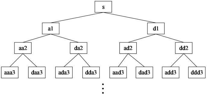
The wavelet packet energy coefficient is an appropriate choice for analyzing the characteristics of acoustic emission signals, allowing for quantification of the frequency features of the signal. The analysis method involves performing a -level wavelet packet decomposition on the detected signals. The signal is then divided into frequency bands, with the -th frequency band defined as , . The original signal is represented as the sum of all wavelet packet components at the -th level:
The energy of the wavelet packet components in the -th frequency band can be expressed as:
The total energy of the signal is calculated as:
The energy coefficient of the -th frequency band is defined as:
In such a manner, illustrates the energy coefficient distribution in each frequency band.
The flow process diagram of WPT is displayed in Fig. 1.
Fig. 1Flow process diagram of WPT
2.2. Principal component analysis
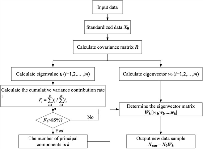
Principal Component Analysis (PCA) is an effective statistical technique to eliminate redundant information efficiently. The frequency band energy values obtained from the Wavelet Packet Transform are multidimensional feature data with strong correlations, which increase the computational load and complexity of data analysis. PCA performs an orthogonal transformation on these highly correlated multidimensional variables, yielding a smaller number of linearly independent principal components. This reduces the number of variables to be analyzed while preserving the maximum amount of information from the original data. The flow process diagram of PCA is described in Fig. 2.
Fig. 2Flow process diagram of PCA
First, the data must be centralized by calculating and removing the mean of each measurement, i.e.:
where is the -th feature of the -th data and is the sample mean.
After centralizing the data, the new data matrix, , is constructed. The next step is to calculate the sample covariance matrix, :
Each element of the covariance matrix R represents the covariance between the -th and -th features. To obtain the eigenvalues and corresponding eigenvectors of the sample covariance matrix , the characteristic equation is solved, which is expressed as follows:
where is a diagonal matrix containing the eigenvalues arranged in descending order, i.e., , with . is s the orthogonal matrix composed of the eigenvectors, with the -th column of being the eigenvector corresponding to the eigenvalue .
Next, the individual variance contribution ratio () and the cumulative variance contribution ratio () for each eigenvalue are calculated using the following formulas:
A larger variance contribution ratio () indicates a stronger ability of the principal component to explain the original variables. The first principal component usually has the largest contribution ratio. Similarly, a larger cumulative variance contribution ratio () corresponds to a greater proportion of the original information captured by the first k principal components. Typically, the first principal components are retained when the cumulative variance contribution ratio reaches 85 %.
Finally, the selected first principal components are used to construct the matrix, and the original data are projected onto the new principal component space as shown below:
3. Experimental
This chapter presents the experimental setup and procedures used to investigate corrosion of Q235 steel under simulated marine conditions. It covers specimen preparation, sensor configuration, and real-time acquisition of acoustic emission (AE) signals. Detailed descriptions of the experimental design are provided to ensure reproducibility and clarity.
3.1. Material and sample preparation
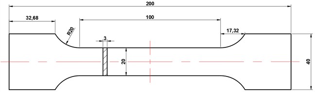
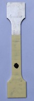
The material used in the experiment is Q235 low-carbon steel, with dimensions as shown in Fig. 3 as illustrated in Fig. 4(a), only a portion of the specimen is exposed to the corrosive environment, designated as the corrosion area, while the remainder of the surface in contact with the solution is covered with an anti-corrosion coating, including both sides and edges, ensuring full coverage. The experimental solution is a mixture of 5 % NaCl and 5 % Na2SO4 by mass, and the container used is a glass beaker.
As shown in Fig. 4(b), a substantial amount of reddish-brown corrosion products, mainly iron oxides, has formed on the specimen surface. Over time, the corrosion product layer thickens and accumulates due to gravity. Eventually, the adhesion between the product layer and the substrate becomes inadequate to support its own weight, causing the layer to peel off and form a downward sliding morphology. This phenomenon indicates that Q235 steel has experienced a relatively severe corrosion process in this environment.
Fig. 3Specimen dimension scheme
3.2. Experimental setup and test method
The acoustic emission detection equipment and α-series sensors from Physical Acoustics Corporation (PAC), USA, were used in the experiment. The threshold value is set at 45 dB to filter out most environmental noise, thus minimizing its impact. The filter range is simulated from 1 kHz to 1 MHz, covering the primary frequency band of the acoustic emission signals. The sampling rate is 1 MHz, and the maximum frequency of the collected acoustic emission signals is 500 kHz. The pre-trigger time is 100 µs, and the sampling length is 1k. The peak detection time (PDT), hit detection time (HDT), and hit lockout time (HLT) are 300 µs, 600 µs, and 1000 µs, respectively. The HLT value ensures that each collected acoustic emission signal avoids interference from reflected and late-arrival waves, capturing only localized changes in the material.
Fig. 4Pretreatment and corrosion samples
a) Pretreatment samples
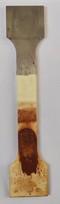
b) Corrosion morphology samples
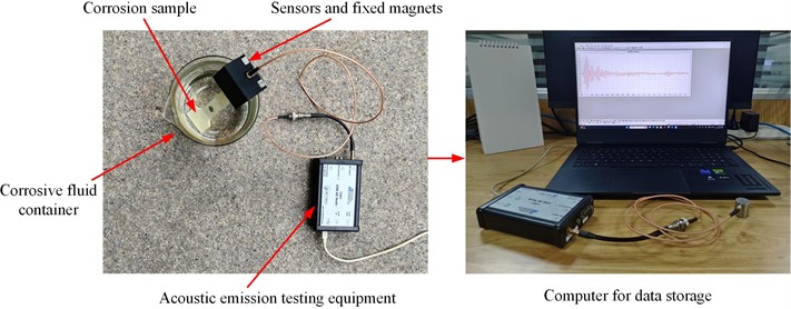
In the experiment, one end of the specimen is immersed in the solution to ensure complete coverage of the corroded area. A fixed magnet is used to position the sensor at the opposite end of the specimen, which is connected to the acoustic emission monitoring equipment and a computer for real-time monitoring of the corrosion signals. The corrosion process was monitored in real time for 10 days. And two parallel experiments were conducted. The experimental setup is illustrated in Fig. 5.
Fig. 5Schematic representation of the experimental setup
4. Results and discussion
This chapter presents research findings using visualizations of signal waveforms, energy distribution maps, and clustering analysis, elucidating the relationship between AE signal features and corrosion mechanisms. Subsequently, the performance of a convolutional neural network (CNN) model in classifying AE signals is assessed, demonstrating its accuracy and potential for real-time corrosion monitoring.
4.1. Feature extraction of AE signals
To investigate the relationship between the AE signals and the microstructural damage of Q235 steel under corrosion environment, 4-level wavelet packet decomposition using the db3 wavelet was applied to each collected AE signal.
For acoustic emission signals, it is essential to choose a discrete wavelet basis with properties similar to those of the signal, such as compact support, orthogonality, and regularity. The db3 wavelet basis meets these requirements and effectively preserves the signal's original features during the wavelet transform. It also performs well in signal compression and reconstruction, ensuring the accuracy of the analysis [25, 26].
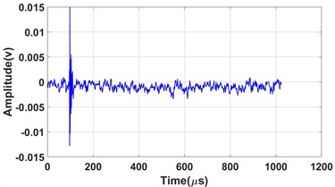
After decomposition, the signals were decomposed into 16 frequency bands, ranging from low to high frequency at each scale, with a bandwidth of 31.25 kHz for each band. The energy coefficients were then calculated to analyze the frequency characteristics of the acoustic emission signals. Fig. 6 presents the typical acoustic emission signal waveform along with its corresponding energy coefficients obtained from the experiment.
Fig. 6The typical acoustic emission signal waveform and its energy coefficients
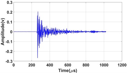
a) Acoustic emission signal waveform
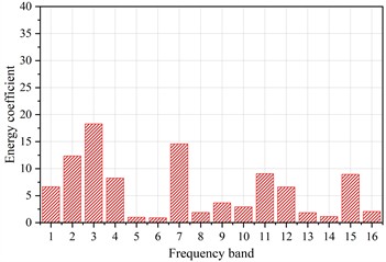
b) Acoustic emission signal energy coefficients
Conducting a correlation analysis prior to cluster analysis enables a straightforward assessment of the degree of correlation among different WPT energy coefficients of acoustic emission signals. The formula for calculating the correlation coefficient between the energy coefficients is as follows:
where is the correlation coefficient, is the covariance between variables and , and is the standard deviation of each of the variables and , to defined as the energy coefficients in the frequency bands 1-16.
The normalized data are substituted into Eq. (10), and the correlation coefficients of the energy values for each frequency band are presented in Table 1.
Table 1Correlation coefficients of the energy coefficients for each frequency band
P1 | P2 | P3 | P4 | P5 | P6 | P7 | P8 | P16 | ||
P | 1.00 | 0.35 | 0.52 | 0.51 | 0.38 | 0.50 | 0.53 | 0.42 | –0.34 | |
P2 | 0.35 | 1.00 | 0.83 | 0.80 | 0.59 | 0.75 | 0.80 | 0.82 | –0.44 | |
P3 | 0.52 | 0.83 | 1.00 | 0.83 | 0.60 | 0.78 | 0.88 | 0.77 | –0.48 | |
P4 | 0.51 | 0.80 | 0.83 | 1.00 | 0.60 | 0.78 | 0.81 | 0.82 | –0.44 | |
P5 | 0.38 | 0.59 | 0.60 | 0.60 | 1.00 | 0.69 | 0.58 | 0.65 | –0.29 | |
P6 | 0.50 | 0.75 | 0.78 | 0.78 | 0.69 | 1.00 | 0.77 | 0.77 | –0.37 | |
P7 | 0.53 | 0.80 | 0.88 | 0.81 | 0.58 | 0.77 | 1.00 | 0.76 | –0.46 | |
P8 | 0.42 | 0.82 | 0.77 | 0.82 | 0.65 | 0.77 | 0.76 | 1.00 | –0.37 | |
P16 | –0.34 | –0.44 | –0.48 | –0.44 | –0.29 | –0.37 | –0.46 | –0.37 | 1.00 |
As shown in Table 1, the correlation between the energy coefficients varies, with certain parameters exhibiting generally higher correlation coefficients, such as those between and , and between and . Therefore, redundant information with high correlation should be eliminated.
PCA was applied to the energy coefficient data of each frequency band to achieve decorrelation and dimensionality reduction. The correlation matrix, eigenvalues, and eigenvectors were calculated, yielding the variance contribution ratios and cumulative variance contribution ratios for each principal component, as shown in Fig. 7.
Fig. 7The individual variance contribution ratios and cumulative variance contribution ratios of each principal component
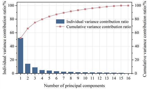
As the number of principal components increases, the growth of the cumulative variance contribution ratio gradually slows. The cumulative variance contribution ratio for the first 6 principal components exceeds 86.96 %, capturing most of the information from the wavelet packet energy coefficients. Therefore, the first 6 principal components are selected as the feature set for each acoustic emission signal, and the original data are projected onto the new principal component space . The eigenvectors corresponding to each principal component are presented in Table 2. The variables to represent the eigenvectors associated with the first six principal components extracted from the covariance matrix.
Table 2The eigenvectors corresponding to each principal component
P1 | –0.2127 | 0.0263 | –0.0639 | 0.8205 | 0.3250 | –0.1531 |
P9 | 0.1569 | 0.4350 | –0.2677 | 0.0680 | –0.3081 | –0.0112 |
P10 | 0.1563 | 0.4455 | –0.3448 | –0.0122 | –0.0715 | 0.2291 |
P11 | 0.2901 | –0.2387 | 0.1437 | –0.0411 | –0.1155 | –0.1683 |
P12 | 0.2044 | 0.4081 | –0.1437 | –0.0930 | 0.2791 | 0.0904 |
P13 | –0.0234 | 0.2058 | 0.6998 | 0.1670 | –0.2753 | 0.3230 |
P14 | –0.1151 | 0.4449 | 0.3806 | 0.0732 | –0.1566 | –0.1236 |
P15 | 0.2990 | –0.2043 | 0.1028 | –0.0602 | –0.1339 | –0.1592 |
P16 | 0.1778 | 0.2185 | 0.3324 | –0.2804 | 0.7255 | –0.1573 |
As illustrated in Table 2, these 6 principal components provide a comprehensive representation of the original data and are relatively independent. The proportions of the energy coefficient parameters are fairly balanced, with no significant bias, indicating that the processing results are satisfactory. The first principal component is strongly correlated with the , , and frequency bands, weakly correlated with the , , and frequency bands, and negatively correlated with the other frequency bands. In the second principal component, the , , , and frequency bands show higher correlations.
Then using as the new matrix, cluster analysis of the signals was performed utilizing the -means algorithm. The acoustic emission signals during the corrosion process are diverse, including signals from pit formation and expansion, bubble rupture, friction, detachment of corrosion products, and film rupture. Among these, the signals resulting from the friction-induced detachment of corrosion products shares a similar generation mechanism with that of the oxide film rupture, both resulting from activities such as creep, friction, and cracking between corrosion products and the membrane layer. Therefore, their signal characteristics are highly similar. Consequently, the number of clusters is set to 3, and clustering is performed on the dimensionality-reduced signals. The spatial distribution of each signal across the first three principal components is shown in Fig. 8. PCA 1, PCA 2, and PCA 3 refer to the first three principal components extracted through principal component analysis.
Fig. 8The spatial distribution of signals for each mode on the first three principal components
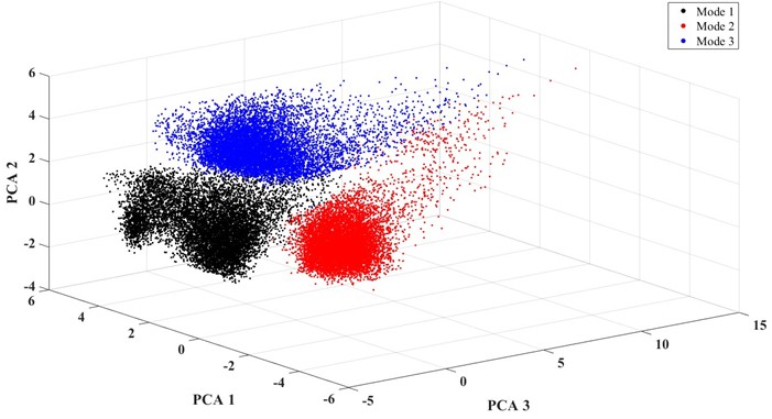
From Fig. 8, it can be observed that there are three signal modes in the corrosion process. The black color represents the signals of Mode 1, the red color represents those of Mode 2, and the blue color represents those of Mode 3. The data of each mode are relatively compact, with clear spatial separation between the modes, indicating good classification results. For signals of mode 1, the first principal component has a larger proportion and is negatively correlated with the third principal component, suggesting that the signals are characterized by a higher proportion of high-frequency bands, specifically the 11th and 15th frequency bands. For signals of mode 2, the first three principal components are more evenly distributed, indicating that the signals in this mode have a significant presence across all frequency bands. Compared to the signals of mode 2, the signals of mode 3 show greater correlation with the first and second principal components, indicating that the energy in the high-frequency bands is higher in Mode 3 than in Mode 2.
4.2. Relationship between AE signals and damage mechanisms correlated with Q235 steel corrosion
Corrosion of Q235 steel materials is a complex process. Chloride ions (Cl⁻) are aggressive and can penetrate the corrosion product film, reacting with the substrate, leading to surface damage and rupture of the film, thereby generating acoustic emission signals. Moreover, corrosion forms pits, and as these pits grow and expand, they also produce acoustic emission signals. Additionally, the accumulation of corrosion products and the friction and shedding between them can generate acoustic emission signals. Furthermore, gas bubbles are continuously formed during the corrosion process, and their rupture generates a small amount of acoustic emission signals.
The wavelet packet transform was applied to signals of different modes to obtain the energy coefficient plot. Typical acoustic emission signal waveforms and energy coefficient plots for three modes are shown in Fig. 9 and Fig. 10.
Fig. 9Waveforms of acoustic emission signals for three typical damage modes: a) mode 1; b) mode2; c) mode 3
a)
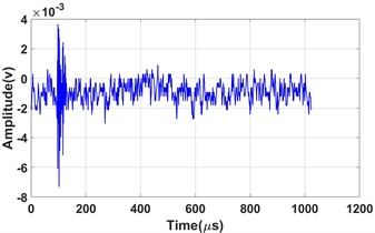
b)
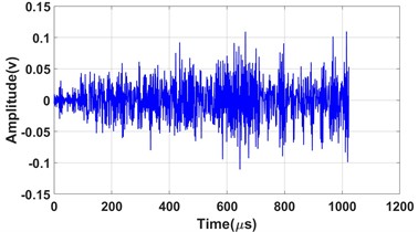
c)
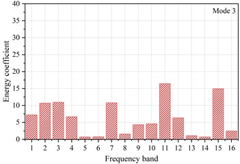
Fig. 10The energy coefficients distribution diagram of signals for three typical damage modes: a) mode 1; b) mode2; c) mode 3
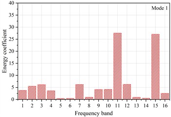
a)
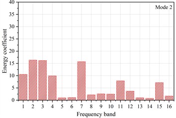
b)
c)
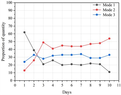
The quantity and variation of these signal for each mode collectively reflect the evolution of the entire corrosion process. By analyzing these variation patterns in detail, the specific signal mode can be determined. Fig. 11 presents the proportion of signals for each mode in each day.
By analyzing the variation in the quantity of signals for each mode in Fig. 11, the corrosion process is divided into three stages: early, middle, and late. During the early stage of corrosion (days 1-3), all signal types undergo changes. The signals of mode 1 decrease, with their proportion dropping from over 60 % on day 1 to around 20 % on day 3. The signals of mode 2 begin with a low proportion on day 1 but increase rapidly over the first three days, rising from 10 % to 50 %. The proportion of signals in mode 3 fluctuates between 20 % and 30 %. During the middle stage of corrosion (days 4-7), the signals of mode 2 consistently have the highest proportion, followed by those of mode 3, while the signals of mode 1 have the lowest. During this period, the signal proportions for all modes remain stable, at approximately 18 %, 48 %, and 34 %, respectively. The stability of all signal modes indicates that the system is gradually reaching equilibrium, and the corrosion process has entered a stable phase.
Fig. 11The proportion of the quantity of signals for each mode in each day
From the Fig 9 and 10, it can be seen that the signal of mode 1 is burst-type, characterized by a short rise time and duration. The energy distribution of this type of signal is relatively concentrated, with the energy proportions in the high-frequency bands of 312-343 kHz and 437-468 kHz both exceeding 25 %. In contrast, the energy proportions in the other frequency bands are all below 7.5 %. Bubble rupture is generally considered to occur instantaneously, lasting only a few dozen microseconds. The rapid release of pressure during rupture generates high-frequency elastic waves [27, 28]. Therefore, the signal of mode 1 is attributed to bubble rupture. In the early stage of corrosion, chloride ions (Cl⁻) in the sodium chloride solution cause localized areas on the Q235 steel surface to corrode, forming small pits or defects. These defect areas serve as the anode in electrochemical reactions, where metal dissolves and releases ions (e.g., Fe2⁺) into the solution. The non-corroded parts of the steel surface serve as the cathode. At the cathode, hydrogen ions (H⁺) are reduced to form hydrogen gas. This reduction reaction generates gas bubbles in the cathodic regions, leading to a higher number of bubble-related signals in the early stages. As corrosion progresses, corrosion products accumulate on the steel surface, slowing the corrosion rate. In addition, the concentration of the corrosive medium decreases due to ongoing reactions, reducing the rate of gas bubble generation and, consequently, the number of rupture signals.
The signal of mode 2 also exhibits burst characteristics, characterized by a slightly longer rise time and duration. The energy of the acoustic emission signal of mode 2 is relatively concentrated in the low-frequency bands, with the energy proportions in the frequency bands of 0-218 kHz reaching 60 %. The AE signal of pit growth is characterized by a short rise time and duration, with fewer high-frequency components. As a result, the signal of mode 2 is attributed to pit growth and expansion. During corrosion, these signals become the primary source of acoustic emissions, with their quantity significantly exceeding that of the other modes. In the early stage of pitting corrosion, the metal surface undergoes localized corrosion, leading to small holes or defects that gradually develop into pits. As corrosion progresses, corrosive ions in the solution react with the metal surface, causing the pits to expand and deepen. During this process, whenever the pit structure changes, such as cracking of the edges, increased depth, or formation of new defects, significant acoustic emission signals are generated. These signals reflect the microscopic damage to the material due to corrosion.
The signal of mode 3 is a continuous-type signal and has a long duration. Its energy distribution is more dispersed, with components present in the mid-to-low frequency bands of 0-125 kHz and 187-218 kHz, as well as the high-frequency bands of 312-343 kHz and 437-468 kHz. Signals from corrosion product shedding and oxide film rupture arise from interactions such as compression, friction, and cracking between the film layer and products, which is a gradual process. Thus, the signal of mode 3 is attributed to the detachment of corrosion products and the rupture of the oxide film. Due to the sample being placed at an inclined angle during the experiment, along with the small amount of corrosion products in the early stage and their weak adhesion in the solution, the corrosion products tend to slide off. What’s more, the mechanism of signals generated by oxide film breakdown is similar to that of signals from the shedding of corrosion products, as both phenomena result from activities such as creep, friction, and cracking between the corrosion products and the film layer. This leads to this mode signal exceeding 20 % in the early stage, with a similar proportion of approximately 32 % in the middle stage.
In the later stages of corrosion, as corrosion products accumulate, the thickness of the product layer gradually increases. This weakens the bond between the corrosion products, causing the previously tightly adhered product layer to become unstable. Large areas of the corrosion product layer begin to peel off, followed by the formation and accumulation of new corrosion products. This peeling phenomenon re-exposes parts of the metal substrate, previously protected by the corrosion product layer, to the corrosive environment, further accelerating material corrosion. This corresponds to the instability of the proportions of signals from different modes in the later stages of corrosion, as shown in Fig. 11. The proportion of mode 2 signals, representing the growth and expansion of pits, continues to increase, while the proportion of mode 1 signals decreases. The proportion of mode 3 signals decreases first, then increases.
4.3. Intelligent monitoring of steel corrosion condition based on convolutional neural network
After performing principal component analysis on the acoustic emission signals, a convolutional neural network (CNN) is applied to establish the nonlinear relationship between the AE signals and damage modes in the other set of experiments. The (CNN) is an architecture that utilizes convolutional layers for feature extraction and pooling layers for dimensionality reduction, combined with fully connected layers for classification. It excels in signal feature extraction and pattern recognition, which is why it has become a crucial tool in this field.
Fig. 12Schematic diagram of the convolutional neural network architecture
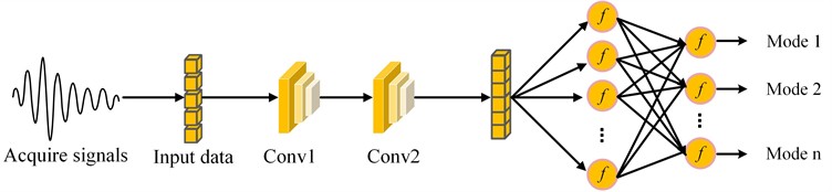
Fig. 12 illustrates the structure of the convolutional neural network adopted in this work. The input layer data comes from the 6 key principal components extracted by PCA. These principal components summarize and represent the core information of the signals. The CNN consists of two convolutional layers and one max-pooling layer. It utilizes the ReLU activation function and produces the final output through a fully connected layer, followed by a Softmax layer and a classification layer. The dataset is randomly shuffled and divided into training and test sets in a 7:3 ratio. The maximum number of iterations is set to 500, and the learning rate to 0.001.
Fig. 13Confusion matrix of the training results
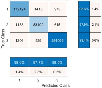
a) Confusion matrix of the training set
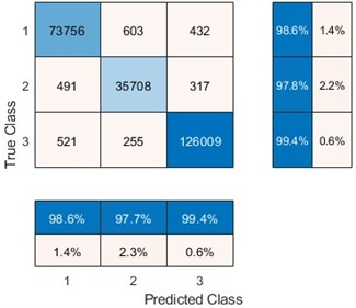
b) Confusion matrix of the test set
Fig. 14Statistical analysis of corrosion damage modes based on convolutional neural network recognition results
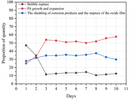
Fig. 13 illustrates the confusion matrix of the convolutional neural network training results. The confusion matrix of the training set shows that with a large dataset, the neural network performs well. The recognition rates for mode 1 and mode 3 signals reach 98.6 % and 99.4 %, respectively, while the recognition rate for mode 2 signals, though lower, still reaches 97.9 %. When applied to the test set, the neural network demonstrates an accuracy of over 97 % in identifying the three damage modes in the acoustic emission signals. This result indicates that the convolutional neural network has excellent self-learning capabilities and strong generalization performance, enabling it to accurately identify different damage modes during the corrosion process based on the acoustic emission signal characteristics. The constructed convolutional neural network was utilized to perform pattern recognition on another set of acoustic emission signals collected during the corrosion process, and the recognition results were statistically analyzed, as shown in Fig. 14. The result provides an intuitive demonstration of the dynamic evolution behavior of Q235 steel during corrosion. The fluctuation in the curve shown in the figure reflects the transition of the corrosion state.
5. Conclusions
In this study, AE technology was used to continuously monitor the corrosion process of Q235 steel plates under simulated marine environment. A correlation between acoustic emission signals and damage mechanisms was established. The main conclusions are as follows:
1) Principal component analysis reduced the wavelet packet energy coefficients of the acoustic emission signals from 16 dimensions to 6, improving classification efficiency while preserving core features. Three distinct acoustic emission signal patterns were identified during the corrosion of Q235 steel applying the K-means clustering method: signals of bubble rupture, pit growth and expansion, and detachment of corrosion products along with oxide film rupture.
2) Signals related to bubble rupture displayed burst-like characteristics, characterized by short rise times and durations. The energy of these signals was mainly concentrated in the high-frequency bands (312-343 kHz and 437-468 kHz). Signals associated with pit growth and expansion also exhibited burst-like characteristics, with slightly longer rise times and durations compared to those from bubble rupture. The energy of these signals were primarily concentrated in the low-frequency range (0-218 kHz). Signals linked to corrosion product detachment and oxide film rupture were continuous, exhibiting longer durations. Their energy distribution was more dispersed, mainly concentrated in the mid-low frequency bands (0-125 kHz and 187-218 kHz) and the high-frequency bands (312-343 kHz and 437-468 kHz).
3) An accuracy of over 97 % in identifying acoustic emission signals is achieved by the established damage mode recognition model based on convolutional neural network. This model exhibits excellent self-learning capabilities and strong generalization performance. The evolution of the corrosion damage in Q235 steel is intuitively presented through statistical analysis of the recognition results output by CNN. This enables real-time monitoring of Q235 steel corrosion condition.
References
-
S. Lu et al., “Extracellular electron transfer corrosion mechanism of two marine structural steels caused by nitrate reducing Halomonas titanicae,” Corrosion Science, Vol. 217, p. 111125, Jun. 2023, https://doi.org/10.1016/j.corsci.2023.111125
-
Y. W. Liu, T. Z. Gu, Z. Y. Wang, C. Wang, and G. W. Cao, “Corrosion behavior of Q235 and Q450NQR1 exposed to marine atmospheric environment in Nansha, China for 34 months,” Acta Metallurgica Sinica, Vol. 58, No. 12, pp. 1623–1632, 2022, https://doi.org/10.11900/0412.1961.2021.00576
-
R. Wang et al., “Influence of stress on corrosion behavior and evolution model of Q235 steel in marine environments,” International Journal of Pressure Vessels and Piping, Vol. 214, p. 105388, Apr. 2025, https://doi.org/10.1016/j.ijpvp.2024.105388
-
Z. Kong et al., “Experimental and theoretical study on mechanical properties of mild steel after corrosion,” Ocean Engineering, Vol. 246, p. 110652, Feb. 2022, https://doi.org/10.1016/j.oceaneng.2022.110652
-
M. A. A. Aldahdooh, N. M. Bunnori, and M. A. Megat Johari, “Damage evaluation of reinforced concrete beams with varying thickness using the acoustic emission technique,” Construction and Building Materials, Vol. 44, pp. 812–821, Jul. 2013, https://doi.org/10.1016/j.conbuildmat.2012.11.099
-
W. Li and G. Palardy, “Damage monitoring methods for fiber-reinforced polymer joints: A review,” Composite Structures, Vol. 299, p. 116043, Nov. 2022, https://doi.org/10.1016/j.compstruct.2022.116043
-
A. Huijer, C. Kassapoglou, and L. Pahlavan, “Acoustic emission monitoring of composite marine propellers in submerged conditions using embedded piezoelectric sensors,” Smart Materials and Structures, Vol. 33, No. 9, p. 095018, Sep. 2024, https://doi.org/10.1088/1361-665x/ad6739
-
W. Zhou, Y.-G. Du, S.-D. Wang, Y.-P. Liu, L.-H. Ma, and J. Liu, “Effects of welding defects on the damage evolution of Q245R steel using acoustic emission and infrared thermography,” Nondestructive Testing and Evaluation, Vol. 38, No. 2, pp. 189–210, Mar. 2023, https://doi.org/10.1080/10589759.2022.2094377
-
F. Wen, Z. Long, Z. Xing, W. Guo, and Y. Huang, “Research on damage behavior of thermal barrier coatings based on acoustic emission technology,” Nondestructive Testing and Evaluation, Vol. 38, No. 1, pp. 67–89, Jan. 2023, https://doi.org/10.1080/10589759.2022.2066665
-
W. Zhou, Y.-Z. Liang, S.-N. Xue, and L.-H. Ma, “Acoustic emission source location for composite tubes using finite element simulation and machine learning,” Nondestructive Testing and Evaluation, Vol. 40, No. 3, pp. 1229–1251, Mar. 2025, https://doi.org/10.1080/10589759.2024.2339541
-
P. Zhang, Q. Lin, S. Li, and J. Wang, “Research on the in situ tensile fracture behavior of Q355E steel and its welded joints based on acoustic emission,” Russian Journal of Nondestructive Testing, Vol. 60, No. 6, pp. 602–613, Sep. 2024, https://doi.org/10.1134/s1061830924600187
-
X. Wei, Y. Chen, C. Lu, G. Chen, L. Huang, and Q. Li, “Acoustic emission source localization method for high-speed train bogie,” Multimedia Tools and Applications, Vol. 79, No. 21-22, pp. 14933–14949, Jan. 2020, https://doi.org/10.1007/s11042-019-08580-3
-
J. Hou, C. Wang, S. Li, N. Jiang, B. Xu, and G. Wu, “Study on propagation mechanism and attenuation law of acoustic emission waves for damage of prestressed steel strands,” Measurement, Vol. 219, p. 113240, Sep. 2023, https://doi.org/10.1016/j.measurement.2023.113240
-
Z. Zhang et al., “In-situ monitoring of pitting corrosion of AZ31 magnesium alloy by combining electrochemical noise and acoustic emission techniques,” Journal of Alloys and Compounds, Vol. 878, p. 160334, Oct. 2021, https://doi.org/10.1016/j.jallcom.2021.160334
-
J. Park, J. S. Kim, D. Y. Lee, and S. H. Lee, “Real-time monitoring of stress corrosion cracking in 304 L stainless steel pipe using acoustic emission,” Journal of Nuclear Materials, Vol. 571, p. 154009, Dec. 2022, https://doi.org/10.1016/j.jnucmat.2022.154009
-
Z. Wang, K. Ding, H. Ren, and J. Ning, “Quantitative acoustic emission investigation on the crack evolution in concrete prisms by frequency analysis based on wavelet packet transform,” Structural Health Monitoring, Vol. 21, No. 3, pp. 1046–1060, Jun. 2021, https://doi.org/10.1177/14759217211018871
-
R. Gutkin, C. J. Green, S. Vangrattanachai, S. T. Pinho, P. Robinson, and P. T. Curtis, “On acoustic emission for failure investigation in CFRP: Pattern recognition and peak frequency analyses,” Mechanical Systems and Signal Processing, Vol. 25, No. 4, pp. 1393–1407, May 2011, https://doi.org/10.1016/j.ymssp.2010.11.014
-
J. G. Ning, L. Chu, and H. L. Ren, “A quantitative acoustic emission study on fracture processes in ceramics based on wavelet packet decomposition,” Journal of Applied Physics, Vol. 116, No. 8, p. 3773, Aug. 2014, https://doi.org/10.1063/1.4893723
-
M. Barbosh and A. Sadhu, “Wavelet packet transformation-based improved acoustic emission method for structural damage identification,” Smart Materials and Structures, Vol. 34, No. 1, p. 015036, Jan. 2025, https://doi.org/10.1088/1361-665x/ad9dc8
-
W. Li, P. Sun, Y. Liu, P. Jiang, and X. Yan, “Tensile damage mechanisms of carbon fiber composites at high temperature by acoustic emission and fully connected neural network,” Materials Testing, Vol. 64, No. 6, pp. 893–901, Jun. 2022, https://doi.org/10.1515/mt-2021-2172
-
J. Wang, W. Zhou, X.-Y. Ren, M.-M. Su, and J. Liu, “A waveform-based clustering and machine learning method for damage mode identification in CFRP laminates,” Composite Structures, Vol. 312, p. 116875, May 2023, https://doi.org/10.1016/j.compstruct.2023.116875
-
J. Zhao, W. Xie, D. Yu, Q. Yang, S. Meng, and Q. Lyu, “Deep transfer learning approach for localization of damage area in composite laminates using acoustic emission signal,” Polymers, Vol. 15, No. 6, p. 1520, Mar. 2023, https://doi.org/10.3390/polym15061520
-
J. Cui et al., “Damage identification and fracture behavior of 2.5D SiCf/SiC composites under coupled stress states,” Materials and Design, Vol. 241, p. 112964, May 2024, https://doi.org/10.1016/j.matdes.2024.112964
-
V. Vy, Y. Lee, J. Bak, S. Park, S. Park, and H. Yoon, “Corrigendum to “Damage localization using acoustic emission sensors via convolutional neural network and continuous wavelet transform” [Mech. Syst. Signal Process. 204 (2023) 110831],” Mechanical Systems and Signal Processing, Vol. 215, p. 111413, Jun. 2024, https://doi.org/10.1016/j.ymssp.2024.111413
-
Y. Wang, S. J. Chen, S. J. Liu, and H. X. Hu, “Best wavelet basis for wavelet transforms in acoustic emission signals of concrete damage process,” Russian Journal of Nondestructive Testing, Vol. 52, No. 3, pp. 125–133, Jun. 2016, https://doi.org/10.1134/s1061830916030104
-
D. Li, Q. Hu, J. Ou, and H. Li, “Fatigue damage characterization of carbon fiber reinforced polymer bridge cables: Wavelet transform analysis for clustering acoustic emission data,” Science China Technological Sciences, Vol. 54, No. 2, pp. 379–387, Feb. 2011, https://doi.org/10.1007/s11431-010-4198-7
-
K. Wu, N. Yatagai, K. Ito, T. Shiraiwa, and M. Enoki, “Direct evidence of hydrogen bubble evolution as an acoustic emission source in metal corrosion,” Corrosion Science, Vol. 240, p. 112429, Nov. 2024, https://doi.org/10.1016/j.corsci.2024.112429
-
K. Wu and J.-Y. Kim, “Acoustic emission monitoring during open-morphological pitting corrosion of 304 stainless steel passivated in dilute nitric acid,” Corrosion Science, Vol. 180, p. 109224, Mar. 2021, https://doi.org/10.1016/j.corsci.2020.109224
About this article

This work was supported by the National Natural Science Foundation of China (Grant No. 12202427) and the Science and Technology Planning Project of Zhejiang Province, China (Grant No. 2023C01163).
The datasets generated during and/or analyzed during the current study are available from the corresponding author on reasonable request.
Zonglian Wang: conceptualization, methodology, investigation, writing-review and editing, funding acquisition. Zihao Meng: investigation, methodology, writing-original draft preparation, software, data curation. Di Wang: methodology, software. Mingxuan Liang: writing-review and editing, resources. Keqin Ding: conceptualization, methodology, investigation, project administration.
The authors declare that they have no conflict of interest.
