Abstract
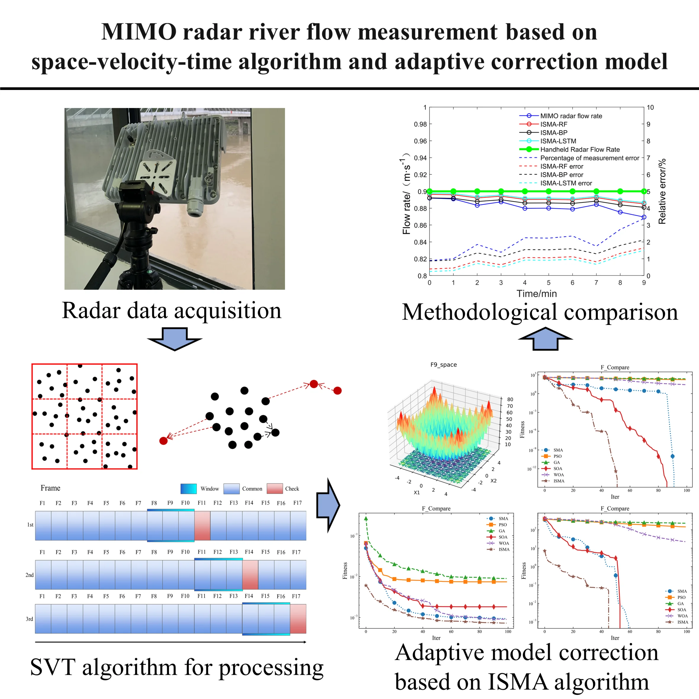
Accurate measurement of river hydrological characteristics is critical for assessing the impacts of flooding caused by meteorological and geomorphological factors. Flow velocity are key indicators in hydrological monitoring. Traditional measurement approaches, such as continuous-wave Doppler radar and pulsed radar systems, are typically mounted on bridges or fixed supports and offer only single-point measurements. These methods often suffer from limited detection range, low accuracy, and poor resistance to environmental interference. To address these limitations, this study proposes a three-dimensional flow detection framework based on multi-input multi-output (MIMO) radar sensors. By leveraging the high reliability and interference resistance of MIMO radar, along with a Space-Velocity-Time (SVT) algorithm that incorporates spatiotemporal information (two-dimensional surface velocity and time), the proposed method enables robust 3D river flow monitoring. In this study, comparative experiments were conducted on four rivers in China with different flow conditions, geomorphic features and weather environments. Results demonstrate that the proposed method achieves a measurement error of less than 5 % compared to acoustic Doppler current profilers (ADCP) and other conventional mechanical approaches, while also offering improved safety and real-time performance. Moreover, an adaptive flow correction algorithm is presented, which uses three optimized prediction models to compute the correction factor and reduces the mean streamflow measurement error to 0.79 % after correction, providing an effective solution for river gauging, flood control and flood resilience.
Highlights
- A high-precision river flow measurement method based on spatial, velocity and temporal information.
- Application of machine learning and deep learning to river flow detection.
- Capturing real rivers to validate the algorithm and designing a real-time update system.
1. Introduction
River discharge is a key parameter in hydrological testing. Due to realistic environmental measurement conditions discharge cannot be measured directly and usually needs to be derived from a combination of integrated surface water level, flow rate and cross-sectional area measurements [1-3]. Cross-sectional profiles are usually obtained from existing bathymetric data or ground-penetrating radar measurements [4-6]. Highly accurate streamflow measurements are therefore essential for the accurate estimation of discharge during flooding and hence for the effective management of flood risk, design of mitigation strategies and development of drainage infrastructure.
Traditional techniques for measuring river velocity often rely on in-situ instruments such as acoustic Doppler current profilers (ADCPs) or current meters positioned within the water column [7]. While ADCPs are effective for direct velocity measurements via wading or boat-mounted deployments, their use becomes hazardous and impractical during flood events or heavy rainstorms [8]. However, velocity profiles during floods are particularly valuable for early warning and hazard prevention, underscoring the need for a safe, real-time, and weather-resilient monitoring approach. Near-field remote sensing has emerged as a viable solution, enabling non-contact observation of river flow under various environmental conditions [9]. Surface velocity radar (SVR), a common near-field method, determines flow velocity by detecting Doppler shifts primarily caused by Bragg scattering [10-11]. A conventional SVR employs one transmitting and one receiving antenna, which restricts it to measuring only the radial component of flow velocity due to its inability to resolve azimuthal information [12]. Although narrow beam widths are used to approximate flow direction, interference from multiple signal sources within the radar footprint can distort the measurements [13]. Moreover, wide rivers often exhibit substantial spatial variability in flow velocities caused by geomorphological, climatic, and hydraulic factors, making single-point SVR data insufficient for capturing comprehensive flow dynamics [14]. Side-mounted bank-based SVR systems extend the detection range but struggle with low-velocity flows, where the Doppler frequency falls below the high-pass filter threshold after projection, resulting in signal loss [15]. To address these limitations, In this paper, a shore-based side-mounted multiple-input multiple-output (MIMO) radar system is proposed, which is capable of accurately measuring river flow rates under different conditions with improved spatial coverage, robustness and measurement fidelity.
MIMO radar enables the acquisition of multiple independent observational signals of a single target and facilitates the fusion of these signals for enhanced target detection [16]. By leveraging radars transmit waveform diversity, MIMO radar provides improved beamforming flexibility, superior detection capabilities, and enhanced interference suppression [17-19]. It also demonstrates a significantly higher sensitivity in detecting slow-moving and weak targets within cluttered environments [20-21]. To leverage the advantages of multi-input multi-output (MIMO) radar in addressing the challenges of river flow measurement, this study proposes a novel three-dimensional point cloud processing algorithm based on the Space-Velocity-Time (SVT) framework. The method exploits the spatial distribution of surface flow velocity within the radar’s field of view (FOV) to suppress and correct signal noise, by incorporating two key domain-specific features: the inherent temporal continuity of river flow and the strong temporal correlation of flow velocity. In addition, an adaptive correction model is developed to dynamically refine the flow velocity measurements, thereby enhancing overall accuracy. The proposed approach enables rapid and precise data acquisition using a single sensor, even under varying environmental conditions, effectively reducing measurement costs while improving operational efficiency.
2. Experimental methods
2.1. MIMO radar point cloud data model
The radar system utilized in this study is the Huawei ASN850 centralized MIMO radar. Operating at a carrier frequency of 80 GHz, the system enables higher Doppler frequency shifts under identical flow conditions, thereby enhancing the sensitivity to velocity changes. It employs an antenna array configuration comprising eight transmitters and eight receivers, which significantly improves angular resolution and measurement accuracy. Furthermore, the radar operates in the frequency-modulated continuous wave (FMCW) mode, providing high range resolution and real-time capability essential for hydrological monitoring.
In a centralized MIMO radar system, the spacing between array elements – or the effective antenna aperture – is considerably smaller than the distance to the target. As a result, each transmitted and received signal observes essentially identical target parameters, including direction of arrival (DOA), range, Doppler frequency, and radar cross section (RCS) [22]. The MIMO radar estimates the target’s distance, velocity, and angle by transmitting FMCW and analyzing the time delay, frequency shift, and phase differences in the received echoes. The ranging process is based on the time delay of the electromagnetic wave traveling from the transmitter to the target and back, combined with the known frequency sweep rate, to compute the range. Velocity estimation is performed by applying fast Fourier transform (FFT) to a sequence of received FMCW pulses and calculating the target speed from the inter-pulse phase differences. Angular estimation is achieved by exploiting the phase differences between signals received across the antenna array, with angular resolution directly related to the number of antenna elements – greater array density yields higher angular precision.
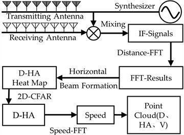
The radar RF chip generates a Chirp signal, which is transmitted through the transmitter antenna and fed into the mixer; the receiver antenna receives the echo signal reflected from the object and transmits it to the mixer to mix with the transmitter signal to form an Intermediate Frequency (IF) signal. FFT is performed on the IF signal in the distance dimension, and the distance-horizontal angle heat map is obtained by beamforming in the horizontal direction, which is processed by 2D-Constant False-Alarm Rate (2D-CFAR) to extract the distance and horizontal angle information of the target. Finally, the velocity dimension Fast Fourier Transform is done to acquire the velocity information [23]. The distance, horizontal angle, and velocity information of target points are gathered by the preceding stages, and the information of numerous target points is assembled into a point cloud and out-put. The MIMO radar signal processing pathway is presented in Fig. 1.
Fig. 1Radar signal processing flow diagram
The IF signal is received by many antennas and physical information such as relative distance, radial velocity and horizontal angle of the target is extracted to generate multidimensional point cloud data which can be represented as:
where represents the relative distance between the target and the radar, represents the radial velocity of the target, satisfies the horizontal angle, and RCS represents the effective radar scattering cross-section area.
When the radar detects the target object, the transmitted signal as well as the received signal after a series of processing will produce multiple point cloud data, which is called point cloud data set and can be expressed as:
2.2. Design of SVT algorithm for 3D point cloud
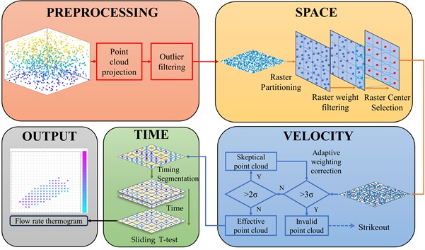
This study presents a point cloud data processing algorithm based on the three-dimensional SVT model, designed for the acquired point cloud dataset. The algorithm leverages physical parameters such as relative distance, radial velocity, and horizontal angle to perform processing tasks, including point cloud clustering and feature extraction, within the three-dimensional space, velocity, and time domains. This approach facilitates the rapid aggregation and streamlined processing of the point cloud data, effectively mitigating noise interference and reducing data redundancy in the river flow measurement. The detailed workflow of this method is illustrated in Fig. 2.
1. Acquisition and Pre-processing of Point Cloud: The MIMO radar system is initialized to capture 3D point cloud data. Based on the radar installation settings, the point cloud is projected onto the horizontal plane. A global adaptive distance thresholding method is then applied to eliminate outlier noise points, thereby reducing interference in the point cloud data.
2. Spatial Dimension Processing: The pre-processed point cloud data is divided into multiple raster blocks according to spatial dimensions. Noisy points are removed by evaluating the weights of points within each raster, optimizing the point cloud data. The center point of each raster is selected to represent the point cloud position, simplifying subsequent data processing.
3. Velocity Dimension Processing: Outliers in the flow velocity data within each raster are corrected and removed using a three standard deviation (3σ) scale correction method. The corrected flow velocity mean value is then assigned to the center point of each raster.
4. Time Dimension Processing: The corrected point cloud data is temporally segmented, with real-time radar data divided into distinct frames, where each frame corresponds to a one-minute interval. A sliding T-test is applied to compare current data with historical data, identifying significant changes. The results are integrated and analyzed to produce the final output.
Fig. 2SVT algorithm flowchart
2.2.1. Preprocessing
Based on the radar shore-based lateral mounting height, pitch, and horizontal angles, and the physical information such as relative distance, radial velocity, and horizontal angle in the point cloud data acquired by the radar system, the point cloud is projected onto the horizontal plane and represented in the form of a matrix:
where the point cloud projection into a 2D coordinate system can be expressed in terms of coordinates and river flow rate:
where represents the relative distance between the target and the radar, represents the radial velocity of the target, represents the horizontal angle measured by the radar, represents the pitch angle of the radar installation, and represents the horizontal angle of the radar installation.
Due to the complex topography of the river, other obstacles such as buildings and vegetation along the banks may interfere with normal signal reception, and floating objects on the surface of the river (e.g., leaves, rubbish, etc.) reflect radar signals and generate echoes that interfere with the water surface echo signals. Therefore, there will be noise points in the initial point cloud produced by radar scanning the river surface [24].
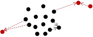
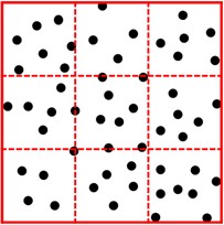
The global adaptive distance thresholding method is applied in the preprocessing to cull out outlier noise points away from the topic point cloud to prevent altering the flow velocity data. Determine the distance threshold based on the global distance average and variance by computing the average of the distance between the target original point cloud and all the points in the neighborhood. When the average of the distance between the point cloud and its nearby points is larger than, the point is declared to be an outlier and rejected. This technique is able to successfully locate and eliminate outlier noise spots, which in turn increases the accuracy of the subsequent processing. As illustrated in Fig. 3, the black dots are the topic point cloud and the red points are the outlier noise points.
Fig. 3Distance thresholding method
2.2.2. Space dimensional point cloud processing
The raster partitioning process is performed on point cloud by traversing each raster and calculating its weights in order to remove redundant points and reduce noise effects. Selecting the center point of the raster to replace the spatial location of the point cloud in the raster further simplifies the number of point clouds, which can more intuitively and accurately show the distribution of flow velocity on the surface of the river.
Dividing the enclosing frame into a number of rasters to improve the accuracy and processing speed of raster clustering. As shown in Fig. 4:
Fig. 4Grid-based partitioning
When the point cloud is denser, the raster edge lengths are smaller to represent the data more finely; when the density is smaller, the raster edge lengths become larger to reduce the computational complexity.
Traverse each raster obtained by the above method in turn, and compute the weights of each point in each raster by means of the neighborhood. The smaller the weight, the denser the distribution of points in the area; conversely, the larger the weight, the more sparsely distributed the points in the area.
For any raster, extract the point with the largest coordinate value and the point with the smallest coordinate value among the points it contains, with initial weights:
where denotes the number of points contained in the raster.
Let a certain matrix contain a set of points , where the weight of any point is:
where denotes the neighborhood of point .
If the weight value of a point in this raster is less than the set weight threshold, the point is rejected, and vice versa, it is retained, thus rejecting the noisy points in the point cloud [25].
In the study of river flow velocity, based on the continuity principle of hydrodynamics and actual observation data, in the gentle section of the river channel, the resistance of the water flow is relatively constant due to the small changes in the riverbed morphology, resulting in small changes in the flow velocity between the proximate points. In addition, the viscosity effect of the fluid makes the flow rate tend to be smoothly distributed over a short range. Thus, the center of the raster is selected to re-place the remaining point-space positions within the raster.
2.2.3. Dimension point cloud processing
The point cloud is stored in a raster through the spatial dimension. In this study, a scaling correction technique based on the law of triple standard deviation is proposed. The method traverses each raster to correct and reject the noise points in the point cloud based on the characteristic that the flow points of the point cloud are normally distributed within the raster. The corrected point cloud flow mean is attributed to the center point of the raster.
Calculation of the average value: By sorting the data and eliminating the very large and very small values in order to exclude the influence of outliers on the average value, so as to obtain a more robust average value. The formula is expressed as follows:
where denotes the average value of the data; denotes the value of the flow rate at the th data point; and denotes the number of data points.
The formula for calculating the standard deviation is expressed as follows:
where is the standard deviation; is the number of data points; and is the th data point.
The weighted correction formula is expressed as follows:
where denotes the flow rate value of the suspected point cloud; denotes the number of suspected point clouds; and denotes the total number of point clouds.
Through iterative processing, the flow velocity data of all point clouds within each raster deviate from the mean value by no more than two times the standard deviation to obtain a single frame of valid point cloud data. Take the average of the point cloud flow rate data in each raster and assign it to the center point of the raster.
2.2.4. Time dimensional point cloud processing
Capturing point cloud features throughout time by separately assessing data collected by the radar in real time at different time periods. Further integrating and analyzing the processing results of each time period can effectively identify and track the dynamic changes of point cloud data.
The point cloud data supplied from the radar in real time is segmented according to the time sequence of one frame per minute, and each frame is processed as a spatial and velocity dimensional point cloud separately. Based on the first ten frames of point cloud data are aggregated and averaged for integrated processing, and each subsequent newly created frame of point cloud data is treated independently. For the current frame, the algorithm takes the data from the previous ten frames as a basis for correcting and evaluating it.
In order to detect whether there is a significant change in the processed single-frame data between different time periods, the algorithm in this research uses a sliding t-test. In this method, the difference between the newly created data and the previous data may be constantly compared every minute, thus improving the accuracy and reliability of data processing.
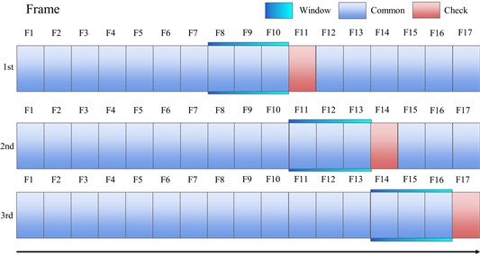
The window size chosen for the sliding t-test algorithm in this study is 11 frames. The window starts from the start position of the time series and gradually slides back 3-5 frames, moving the window until it covers the entire time series. For each window position, the data within the window is divided into two parts (the first 10 frames and the last 1 frame), and a t-test is performed on the two parts of the data to calculate the t-statistic and p-value. As shown in Fig. 5.
Fig. 5Schematic diagram of sliding t-test
Based on the T-statistic and P-value, it was determined whether there was a significant change in a particular window location. If the P-value is less than a preset level of significance, the window location is considered to have an anomalous flow rate point, which is weighted and corrected according to the actual situation in the field.
2.3. Adaptive correction model
The river surface fluid state is unstable due to geomorphic features, environmental factors, weather, and fluid interactions, and although the SVT algorithm can be used to remove some of the noise during detection, there are still nonlinear disturbances caused by a variety of river features.
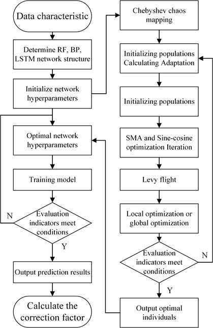
To further improve the accuracy of radar-measured flow velocity, an adaptive flow velocity correction model is proposed. Using machine learning and deep learning methods, river features, weather features, signal features, etc. are used as model inputs, and random forest method, BP network and LSTM network are used to predict the river flow rate, calculate the correction factor, and search for the hyper-parameters of the three models by designing an improved slime mould algorithm (ISMA) to accelerate the convergence speed and avoid falling into the local optimal solution [26]. Meanwhile, in order to meet the real-time river detection, the segmented incremental learning method is used to iteratively update the correction factor to improve the model accuracy and robustness. The detailed model principle is shown in Fig. 6.
Fig. 6Optimization model structure diagram
2.3.1. ISMA
2.3.1.1. Slime mould algorithm (SMA)
SMA is to search for the optimal parameter combinations by imitating the foraging process of Sticky Mushroom, which makes the model efficiency improve [27], and the iteration idea is as follows:
where: and are random numbers between [0, 1]; and are the upper and lower boundaries of the table search range; are the position update parameters; and are the parameters of the slime mold oscillations, and are the random numbers between , where , and are the current iteration number and the maximum iteration number, respectively, and are the random numbers between [–1, 1]; is the algorithm control parameter, and the value of which is related to the fitness value of the algorithm; is the slime mold location, which is superscripted as the number of iterations. is the current best position, and are the positions of two randomly selected individuals at time . The number of iterations is the number of iterations.
2.3.1.2. Chebyshev chaotic mapping
In the early step of the optimization procedure, the original population needs to be initialized. In order to prevent the algorithm from maturing prematurely and having a single population, Chebyshev chaotic mapping is utilized to improve the uniformity and diversity of the initialization of the population [28]. The principle is:
where is the population individuals and is the number of iterations.
2.3.1.3. Sine-cosine optimization
In order to increase the convergence speed of the model, improving the real-time performance of the algorithm is crucial for flow rate detection. Optimizing the SMA by the periodic characteristic of the Sine-cosine optimization algorithm can realize the global and local search of the optimal parameters, jumping out of the local optimum and improving the accuracy [29]. The updating principle is as follows:
where is the solution of the th individual at generation , is the current global optimal solution, and is a randomization factor.
2.3.1.4. Levy flight
Combining sine-cosine optimization may also limit its search capability due to the iteration step size. Using levy flight provides non-uniform large step size jump search at different scales to prevent falling into local optimum [30]. Levy flight principle is:
where is the scaling factor, obeys the normal distribution, and is the levy index.
2.3.2. Baseline forecasting model
2.3.2.1. Random forest (RF)
Due to the simple qualities of the input data, the volume of data is moderate. The application of random forest algorithm has excellent accuracy, high operational efficiency, re-duces the risk of overfitting and enhances prediction stability [31].
Random forest improves prediction performance by constructing multiple decision trees and integrating the prediction results. In constructing the decision trees, the Gini index is used as a splitting criterion to split the data and the three-dimensional features of space, time and speed are used for training. Gini index principle:
where is the probability that category is at the current node . A smaller Gini index indicates a higher purity of the dataset.
Integrating the prediction results of multiple decision trees reduces overfitting, and prediction errors generated by a single decision tree can be corrected by other trees, which in turn improves the robustness of the algorithm. The prediction principle is shown below:
where represents the number of decision trees and represents the prediction result of the th tree.
Also, because to the simple structure of the model, the hyperparameters are easier to define and are suited for use in the early phases of the river when a sufficient quantity of data has been acquired.
2.3.2.2. Back propagation (BP)
As the volume of radar-collected flow rate data increases, environmental factors – such as localized winds on the river surface and small-scale eddies-introduce biases that are difficult to eliminate. These influences contribute to nonlinear relationships among data features, often leading to errors when using random forests due to their reliance on multiple decision trees. To enhance prediction accuracy in this context, a Backpropagation (BP) neural network is adopted. The model computes outputs through forward propagation, while weights and biases are iteratively adjusted using backpropagation [32]. The weights and bias updates are related to the learning rate, and the associated hyperparameter settings are configured using the optimization algorithm below, with the update principle:
where represents the loss function, i.e., the mean square error (MSE).
2.3.2.3. Long short-term memory (LSTM)
The river has continuity, therefore its flow rate changes are strongly tied to time. LSTM network deals with time series data by creating forgetting gates, input gates and output gates to forecast the future flow rate trend based on prior data, which is appropriate for accumulating more time data, real-time correction or abnormal flow rate alert [33].
The core of the LSTM network is the forgetting coefficient and the memory unit, which is updated by iteratively updating the forgetting coefficient and subsequently the memory unit to anticipate the flow rate data. The forgetting coefficient is determined from the current input and the hidden state of the preceding moment:
where , is the weight bias, is the sigmod activation function, and is a value between 0, 1 indicating the degree of forgetting.
The principle of updating the memory unit is as follows:
where is the memory unit.
2.3.3. Adaptive incremental learning strategies
Random Forest and BP both utilize single-point prediction to take the average value, and LSTM uses trend prediction to take the average value as the correction factor to fit with the flow rate detected by radar. The weighting ratio depends on the entire amount of current data for dynamic adjustment. If the entire amount of data in the unit grid after filtering exceeds the threshold, the weighting of the correction factor is in-creased, and a three-level threshold is set, with the maximum not exceeding 0.5.
The three approaches have varied running times when updating the model, and the optimization time for updating the hyperparameters is also diverse, thus the model needs to be partially updated according to the actual use. The random forest approach has a shorter running time and can be updated as a whole with multi-unit and multi-frequency. The BP and LSTM have a longer running period and the update window time can be prolonged to half an hour update or longer.
3. Measurement comparison experiments and calibration of results
3.1. Radar shore-based side mounting
In order to gain higher precision of speed measurement, there are commonly two techniques of placing classic radar flowmeters: bridge center mounting and shore-based telescopic pole mounting, as shown in Figs. 7(a) and 7(b).
Fig. 7Radar installation method
a) Central bridge installation
b) Shore reach pole installation
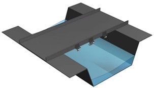
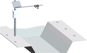
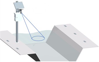
Mounting the radar at the center of a bridge is the most effective setup for capturing the maximum Doppler frequency in areas like Central Sichuan. However, not all monitoring sites are equipped with bridges. Alternatively, shore-based pole installations can still provide a wide radar cross-section and strong Doppler signals. That said, these installations are limited by the spacing between poles, and when the river’s water level drops, the radar beam may no longer reach the water surface effectively. The algorithm proposed in this study is not limited to vertical installations; it also supports lateral mounting on riverbank risers, where the radar is tilted to illuminate the water flow direction at an angle, as shown in Fig. 8.
Fig. 8Shore-based lateral installation
3.2. Signal noise processing
The raw data collected by the radar is affected by environmental factors, there will be a large number of noise signals, so the collected data need to be denoised and filtered [34-36]. The SVT algorithm in this paper can quickly filter out and correct the noise to obtain a more stable set of measurement results. Here we take the 753 flow points with grid coordinates of (39, 19) in Xi’an inner river as an example to show the effect of denoising by SVT algorithm, as shown in Fig. 9.
Fig. 9SVT algorithm denoising effect
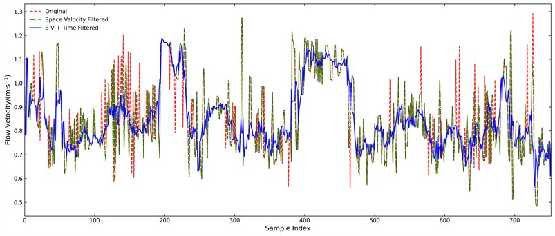
The red dashed line in the figure represents the original data, the green line corresponds to the data after spatial and velocity-domain filtering, and the blue line reflects the results after incorporating temporal-domain filtering. It is evident that the proposed filtering process effectively eliminates abrupt outliers in flow velocity, resulting in a smoother and more consistent temporal trend. Nevertheless, minor fluctuations remain in the filtered data due to environmental, hydraulic, and meteorological influences. However, it is already possible to achieve a decent accuracy in engineering measurements.
3.3. Medium to high flow rate scenarios
Medium and high flow rate scenarios feature strong water surface ripples and waves, making the RCS huge, and the same hardware parameter settings are prone to echo saturation, which introduces high harmonics and interference and leads to unreliable measurement findings.
1. Jinkou River Hydrological Station, Leshan, Sichuan: The MIMO radar is located 14 meters upstream of the cable radar, 27 meters from the cable radar line, 9 meters downstream from the elevation, with a pitch angle of 77° and a horizontal angle of 65°. The SVT calculation results are shown in Fig. 10.
According to Fig. 10, the flow velocity of the Jinkou river is about 4 m/s, which reaches its maximum at a location about 20 meters from the river bank and diminishes at a position far from the river bank. The cableway survey line connects nicely with the radar FOV coverage of only 40 and 50 meters. The flow velocities at the 40 m and 50 m points of the cable radar were 3.90 m/s and 3.86 m/s, respectively, which are com-pared with the flow velocities at the cable radar points as shown in Figs. 11.
Fig. 10Jinhou river SVT algorithm processing result
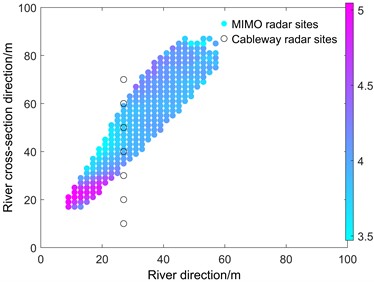
Fig. 11Comparison of flow velocity at Jinkou River measurement points
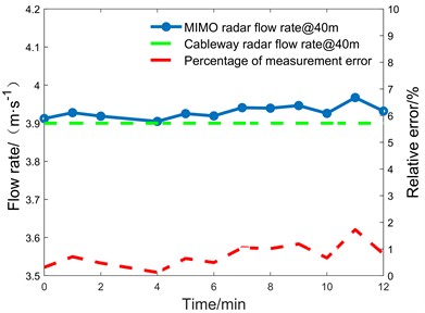
a) Comparison of 40 m measurement points
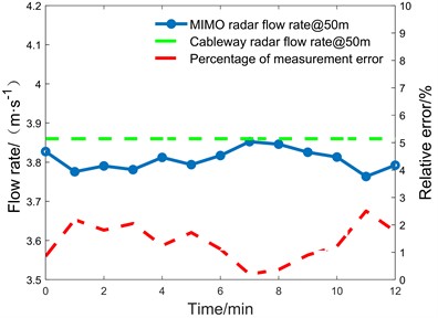
b) Comparison of 50 m measurement points
2. Qinghe River, Beijing: In the experiment, the MIMO radar was positioned at the head of the bridge, looking upstream, at a height of 8 meters from the water level, with a pitch angle of 78° and a horizontal angle of 30°. The radar installation location is shown in Fig. 12(a), and the results of SVT algorithm processing are shown in Fig. 12(b).
Fig. 12Qing river measurement results
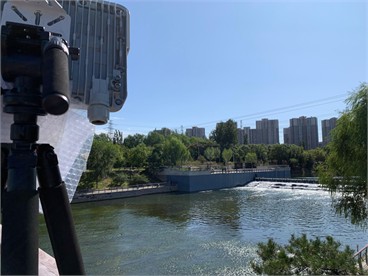
a) Radar installation and deployment at Qing river
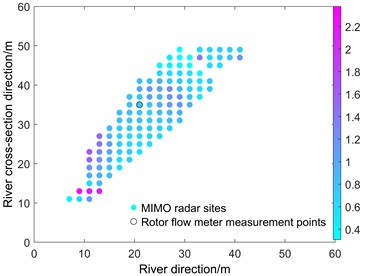
b) Qing river SVT algorithm processing result
According to Fig. 12, it can be seen that the flow velocity of the Qing River in Beijing is about 0.8 m/s, and there is a dramatic increase in the flow velocity at a position about 12 meters from the river bank. It was found that the flow rate in the river channel rose at this point, perhaps due to gullies and hydrilla, while at other areas the flow rate stabilized. As shown in Fig. 13(a), we used a rotameter to estimate the actual flow rate at the site due to the shallow water level of the river, and the comparative results are shown in Fig. 13(b).
Fig. 13Qing river comparison experiment
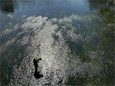
a) Measurements using a rotor current meter
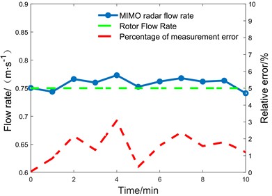
b) Flow velocity comparison at measurement points
3. Xi’an inland river: MIMO radar installed on the bridge, facing downstream, at a height of 15.7 meters above the water surface, with a pitch angle of 78° and a horizontal angle of 30°. The results of the SVT algorithm are shown in Fig. 14(a), and the results of the comparison experiment using the handheld radar are shown in Fig. 14(b).
Fig. 14Xi’an inland river comparison experiment
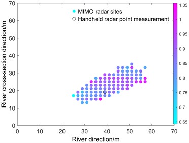
a) Xi’an river SVT algorithm processing result
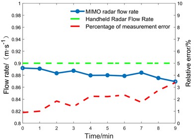
b) Flow velocity comparison at measurement points
Table 1Comparison of flow velocity at medium to high-flow sites
Site | Measurement point coordinates / m | Station flow measurement methods | Site truth value / (m·s-1) | SVT algorithm processing / (m·s-1) | Mean error / % | Maximum error / % |
Jinkou | (27, 40) | Cableway radar | 3.900 | 3.963 | 1.6 | 3.8 |
(27, 50) | 3.860 | 3.789 | 1.8 | 5.0 | ||
Qinghe | (21, 35) | Rotor | 0.751 | 0.758 | 1.5 | 3.08 |
Xi’an | (39, 19) | Handheld radar | 0.900 | 0.882 | 1.98 | 3.39 |
As can be seen from Table 1, the flow velocity findings generated from the 3D point cloud processing algorithm processing were compared with cable channel flow meter radar, rotor type flow meter, and handheld radar flow meter in the experiment.
1) In the experiment at Jinkou river in Sichuan, the flow velocity at the two measurement points was 3.963 m/s and 3.789 m/s by the three-dimensional point cloud processing algorithm, and the average error was less than 2 % compared with the cable radar flow velocity measurements of 3.900 m/s and 3.860 m/s. Cable-channel radar is often used for hydrological monitoring, where streamflow measurements are made by fixing the radar equipment through a cable. They are expensive to build, have poor real-time performance, require regular maintenance of the cableway, and the length and height of the cableway limit their monitoring range. Compared to cable-based radar, shore-based side-scan MIMO radar offers real-time monitoring, is easy to install while providing larger coverage, is not bound by cable lengths and river conditions, and does not require costly cable maintenance.
2) In the experiment on the Qing river in Beijing, the real flow velocity was measured by a rotor-type tachometer, and the result was proved to be 0.751 m/s. At the same measurement position, the flow velocity detected by the MIMO radar was 0.758 m/s, with an average error of 1.5 percent. The rotor flow meter has good measurement accuracy, but it is greatly impacted by water conditions and other factors, confined to detecting the flow velocity at a single spot, and complex to install and maintain. Shore-based side-scan MIMO radars are straightforward to install, are not influenced by water conditions, and give steady measurements in a variety of severe settings.
3). In the experiment of Xi'an inner river, the flow velocity was measured to be about 0.882 m/s by the three-dimensional point cloud processing method, whereas the flow velocity recorded by the hand-held radar flow meter was 0.9 m/s, with an average error of less than 2 %. Handheld radar flowmeters usually can only measure the flow velocity at specific points on the surface of the water body, and it is difficult to obtain the flow velocity distribution information of the whole river area, which is poor in real time, and the measurement results are easily affected by the operator’s station position, angle, and handheld stability, resulting in unstable data or large errors.
By comparing with different traditional flow rate measurement methods at each site, this approach is easy to install, minimizes the demand of the installation environment, and lowers the installation cost and complexity. Able to achieve continuous real-time monitoring, suitable for dynamic changes in the water flow environment, you do not need to be in direct contact with the water body, to reduce the impact of floating objects in the water body, sediment, or water surface fluctuations, to ensure more stable measurement results. At the same time, it is possible to measure the flow velocity distribution at several sites throughout the river channel or a vast area of water instead of being confined to a single point measurement, which is suited for complex river environments.
And through the three-dimensional point cloud processing algorithm, the MIMO radar has a high measurement accuracy; the algorithm processed flow velocity compared with the true value of each site; the average error is less than 2 %; the maximum error is less than 5 %, in line with the industry's requirements for the relative error of less than 5 %.
3.4. Low flow rate scenario
In low flow river scenarios, the radar IF filter circuit must be set up with a high-pass isolation filter, and at the same time, the RCS is small in low-flow, the echo signal is weak, and the signal-to-noise ratio of the low-frequency signal obtained from the sampling is low, which can easily lead to inaccurate measurement values or no measurement results.
Shanxi Bai river hydrological station: The MIMO radar is installed in the well tower, facing upstream, at a height of 19 meters from the water surface, with a pitch angle of 74° and a horizontal angle of 55.7°. The radar is installed and deployed as shown in Fig. 15(a), Rainfall occurred on the day of the experiment, due to rainwater striking the surface of the river to form certain ripples, it will have some impact on the surface flow rate measurement. And due to the rainfall that caused the upstream water level to rise, the upstream gate was opened to release water, resulting in the flow rate result of the measuring point at the downstream location being large. The results of the 3D point cloud processing algorithm are shown in Fig. 15(b).
Fig. 15Bai river measurement results
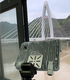
a) Radar installation and deployment at Bai river
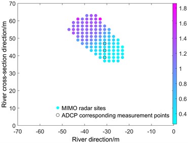
b) Bai river SVT algorithm processing result
According to Fig. 15, the flow velocity at the near-shore point of the Bai river is about 0.4 m/s. The flow velocity at the far-shore point is high due to the reflux of the river water caused by the collision with the bridge abutment. The measurements were compared with the on-site shipboard ADCP, and the ADCP measurements are shown in Fig. 16:
Fig. 16Measurement results from vessel-mounted ADCP
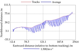
a) Trajectories and flow vectors
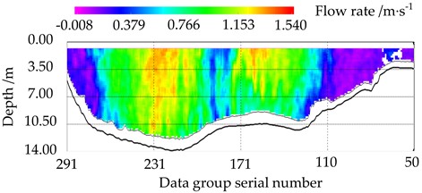
b) Earth coordinate flow velocity magnitude
There are three measurement points, 39 m, 43 m, and 47 m, within the measuring ship course and radar FOV coverage, which are compared with the flow velocity of ADCP, and the results are shown in Fig. 17.
Table 2Comparison of flow velocity at low-flow site
Site | Measurement point coordinates / m | Station flow measurement methods | Site truth value / (m·s-1) | SVT algorithm processing / (m·s-1) | Mean Error / (m·s-1) | Maximum error / (cm·s-1) |
Shanxi Bai river | (–29, 39) | ADCP | 0.296 | 0.314 | 0.018 | 4.04 |
(–29, 43) | 0.241 | 0.261 | 0.020 | 3.78 | ||
(–29, 47) | 0.463 | 0.475 | 0.012 | 2.88 |
According to Table 2, it can be shown that the Shanxi Bai river site employs ship-board ADCP to measure the flow velocity, and the shipboard ADCP detects the water flow information using acoustic wave, and the measurement accuracy is high. But ADCP measurements need the vessel to travel along the survey line, which does not give real-time, full-time monitoring data and is expensive to install and operate. Through the three-dimensional point cloud processing algorithm, the three measurement points measured the flow velocity of 0.314 m/s, 0.261 m/s, and 0.475 m/s, while the flow velocity measured by the ADCP was 0.296 m/s, 0.241 m/s, and 0.463 m/s. The flow velocity processed by the algorithm in the low flow velocity scenario is less than 5 cm/s in comparison with the true value of the site under the absolute error, which is in line with the industry's criteria. Tests have shown that at low flow rates, the approach can give real-time accurate data faster and at cheaper installation and maintenance costs.
Fig. 17Comparison of streamflow at Bai river gauging sites
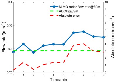
a) 39 m measurement point of Bai River
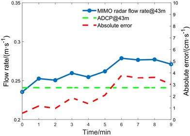
b) 43 m measurement point of Bai River
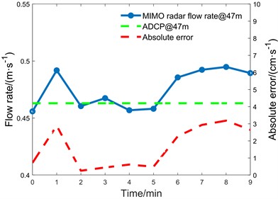
c) 47 m measurement point of Bai River
3.5. Adaptive correction flow rate experiment
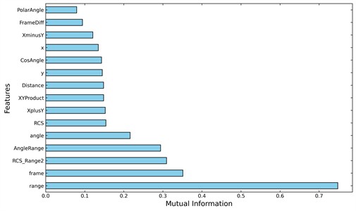
In the above experiments, the data from Xi'an station met the requirements of the algorithm, so adaptive correction experiments were conducted to detect the flow velocity there. A total of 145 887 data were obtained from the experimental data, and three models were used for prediction training, and the data set was divided according to the ratio of 8:1:1. The original features of the river and the enhanced features after feature engineering are shown in Table 3. It contains 7 original features and 9 enhanced features totaling 16 features.
A combination of mutual information, Pearson and Spearman correlation analyses, along with feature–target scatter plots, was used to evaluate feature relevance. After cross-validation, the following features were retained: range, frame, RCS_Range2, Angle Range, angle, Frame Diff. Where , as a core feature of the SVT algorithm is also preserved. Mutual information is analyzed as shown in Fig. 18.
3.5.1. Comparison of optimization algorithms
Fast search configuration of hyperparameters of benchmark models RF, BP, LSTM using optimization algorithms. Among them, RF needs to configure the number of decision trees, the maximum depth of the tree, the maximum number of separated samples, the number of leaf node samples and the maximum number of separated features, and BP needs to configure the activation function, the learning rate, the number of neurons and the number of layers, etc., and the two belong to the low-dimensional search problem. While LSTM needs to configure nearly 30 hyperparameters such as the number of layers, batch size, learning rate, etc., which belongs to the high-dimensional search problem. Therefore, CEC test functions are used to compare multiple optimization models, some test functions are shown in Table 4, and the test results are shown in Fig. 19.
Table 3Characteristic table
Characteristic classification | Feature name | Calculation method | Explanation |
Original features | frame(f) | – | The frame in which the radar collects data |
range | – | Target distance measured by radar | |
v | – | Flow rate detected by radar | |
angle | – | Angle of radar to target | |
RCS | – | Radar Cross section | |
– | Coordinates of the target in space | ||
– | |||
Enhanced features | Distance | Euclidean distance from target to radar origin | |
Cos Angle | Flow velocity versus radar direction | ||
RCS_Range2 | RCS / range² | Reflective intensity per unit distance | |
Angle range | angle*range | Joint characterization of angle and distance | |
Frame diff | Sequence of back minus front frames | ||
Product | Revealing coordinate distribution | ||
plus | Goal-oriented | ||
minus | Target-directed | ||
Polar angle | Target polar angle direction |
Fig. 18Characteristic mutual information analysis
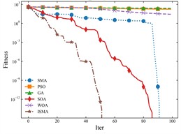
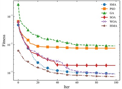
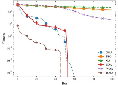
The three test functions listed above correspond to the effect of each algorithm in high-dimensional search under the condition of different variable range sizes, which is to simulate the situation that there are different value ranges in the hyperparameter configurations, e.g., the configuration of the learning rate only needs a single-digit range, while the number of neurons needs a tens or even hundreds of ranges, and in low-dimensional search, the individual algorithms have similar results. The global optimum of all three algorithms is 0, so the closer the fitness of the curve is to 0, the better the search is indicated. The fewer the number of iterations, the more efficient the search is indicated. Therefore, one of the actual search processes in the experiment is extracted and compared, and the comparison effect is shown in Fig. 20.
Table 4Test function
Function name | Function expression | Dimension | Variable range values | Global optimum |
F9 | 30 | [–5.12, 5.12] | 0 | |
F10 | 30 | [–32, 32] | 0 | |
F11 | 30 | [–600, 600] | 0 |
Fig. 19Comparison results of optimization algorithms
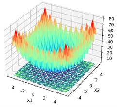
a) F9 test function
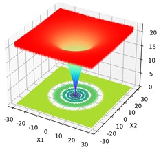
b) F10 test function
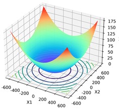
c) F11 test function
d) F9 test results
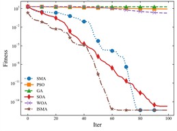
e) F10 test results
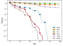
f) F11 test results
Fig. 20Comparison of low and high dimensional real search
a) Comparison of low-dimensional BP search
b) Comparison of high-dimensional LSTM search
As can be seen from the figure, the ISMA method effect has some advantages for both high and low dimensional searches. Therefore, ISMA is finally chosen as the optimization algorithm for the adaptive correction model.
3.5.2. Practical application
30 sets of parameter search experiments were conducted for the three models using ISMA, with the upper limit of 200 iterations for each set and the convergence threshold of 1e-5. The average values of the optimal parameters were calculated to generate the correction factors. The calibration results are shown in Table 5.
Table 5Comparison of three methods of training and results
Methods | Training MAE / (m·s-1) | Training MSE / (m2·s-2) | Calibration factor / (m·s-1) | Target error / % |
ISMA-RF | 0.041316 | 0.0025412 | 0.90093 | 0.93 |
ISMA-BP | 0.039810 | 0.0021796 | 0.89243 | 1.41 |
ISMA-LSTM | 0.040490 | 0.0022191 | 0.90366 | 0.79 |
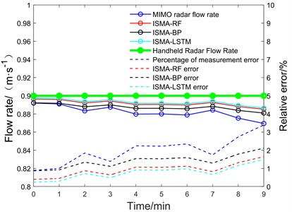
The same scene of Fig. 14 was selected as the target test set, and the flow rate was fitted using the above correction factors, and the results are shown in Fig. 21.
As can be seen from the figure, the flow rate accuracy is improved after correction by all three algorithms, with the most obvious effect being the LSTM network, thanks to its strong correlation with time, followed by Random Forest, and finally the BP algorithm.
Fig. 21Calibration results of the three algorithms are plotted
3.5.3. Time complexity analysis and measurement
The SVT algorithm comprises three main stages: spatial outlier removal, differential smoothing of flow velocity, and temporal filtering via a sliding window t-test. For the spatial filtering step, a triple standard deviation rule is applied within each raster of the point cloud, assuming that the streamflow data approximately follows a normal distribution. Given a total number of flow velocity measurements , and the number of spatial rasters 𝐺, the average number of points per raster is . The complexity of computing the mean, standard deviation, and subsequent replacement for each raster is . The differential smoothing process involves traversing each point and checking adjacent values, which also results in complexity. Similarly, the temporal filtering with a fixed-size sliding t-test window incurs a computational cost of .
The adaptive correction module, which incorporates the ISMA, introduces additional computational overhead. Its complexity depends on the population size , the number of iterations , and the training cost , resulting in . The cost varies based on the underlying prediction model. For example, a Random Forest model with estimators has complexity 𝑂(𝑛_𝑒𝑠𝑡𝑖𝑚𝑎𝑡𝑜𝑟𝑠⋅𝑁⋅log; a Backpropagation Neural Network (BP) with hidden layer size and number of training epochs has complexity ; and an LSTM model, where the sequence length is and the number of hidden units is , incurs a complexity of . Therefore, the overall worst-case computational complexity for the complete algorithmic pipeline, considering ISMA-based optimization and LSTM modeling, is .
To further discuss the real-time performance of the algorithm, a test was conducted using Xi’an inner river data, and the test results are shown in Table 6. The test environment is Intel i5-13500hx and RTX 4060 laptop. The size of the test dataset is 145877×16, the ISMA population is set to 30, the maximum number of iterations in a single run is 100, and the number of runs is 30.
Table 6Algorithm runtime testing
Methods | Runtime / min | Incremental time / s |
ISMA-RF | 3.6 | 234 |
ISMA-BP | 8.2 | 1.8 |
ISMA-LSTM | 13.4 | 7.5 |
Performance evaluation indicates that the ISMA-RF model achieves the shortest runtime, followed by the ISMA-BP neural network with moderate computational demands, while the ISMA-LSTM model incurs the highest computational cost. Notably, the Random Forest (RF) model requires complete retraining upon each update, resulting in progressively longer incremental processing times as the data volume increases. Nevertheless, the runtime of all models remains within acceptable limits for practical engineering applications, thereby demonstrating that the proposed method retains a satisfactory level of real-time applicability.
4. Future research programs and prospects
While the current study is based on short-term measurements recorded in minutes, future work will incorporate extended monitoring campaigns to improve temporal representativeness. A long-term measurement plan will be established with the following considerations: (1) Measurement Duration: Continuous flow velocity data will be collected over extended periods – ranging from several hours to multiple days or weeks – to capture diurnal, meteorological, and seasonal variations. (2) Sampling Frequency: Data will be recorded at fixed intervals (e.g., 1-minute resolution) to ensure consistency with short-term datasets and to facilitate high-resolution temporal trend analysis. (3) Environmental Conditions: Monitoring will be conducted under diverse hydrological and environmental scenarios, including rainfall events, tidal fluctuations in estuarine areas, dry weather periods, as well as challenging contexts such as ice-covered surfaces, sediment-laden flows, and wave-affected zones. These variations will help evaluate the robustness and adaptability of the proposed algorithm. (4) Power and Storage Requirements: To enable autonomous and uninterrupted data acquisition, the system will be supported by solar-powered modules and edge computing devices capable of local data processing and storage. (5) Validation: Periodic cross-validation against reference instruments (e.g., ADCP) will be conducted to ensure measurement reliability and accuracy.
This long-term monitoring strategy is designed to enhance the generalizability and environmental resilience of the proposed approach and to offer a comprehensive understanding of flow dynamics under real-world riverine and estuarine conditions.
5. Conclusions
A Space-Velocity-Time (SVT) point cloud processing algorithm based on MIMO radar is proposed in this study to enhance streamflow measurement accuracy through the integration of spatial distribution, velocity field, and temporal continuity. The algorithm suppresses noise and corrects unstable signals by leveraging the physical characteristics of river flow, such as its gradual spatial variation and temporal correlation. Field validation experiments were conducted in four rivers across China with distinct hydrological conditions, including low-, medium-, and high-flow regimes. Results show that the proposed method provides high-precision monitoring across diverse scenarios. In medium-to-high flow conditions, the deviation between SVT estimates and ground truth values remains below 5 %, and this error can be reduced to 0.79 % through an adaptive correction model. The absolute error is consistently below 0.1 m/s, significantly outperforming previous studies such as [37], which reports an error of 0.24 m/s under similar high-velocity conditions. In low-flow regimes, the maximum absolute error is no greater than 5 cm/s, with an average around 0.02 m/s, showing improvement over the 0.03 m/s reported in [38].
Compared with conventional methods such as Acoustic Doppler Current Profilers (ADCP), rotameters, and cable-based radar, the proposed approach offers advantages in ease of deployment, real-time operability, wide spatial coverage, and reduced maintenance costs. It also demonstrates superior accuracy relative to emerging techniques such as UAV-based or image-based surface flow detection. In summary, the proposed method not only improves the precision and stability of river flow measurements but also provides a scalable and real-time solution applicable to complex field conditions, offering valuable technical support for hydrological monitoring, early warning, and flood disaster mitigation.
References
-
A. Adib et al., “A new approach for suspended sediment load calculation based on generated flow discharge considering climate change,” Water Supply, Vol. 21, No. 5, pp. 2400–2413, Aug. 2021, https://doi.org/10.2166/ws.2021.069
-
L. N. Gunawardhana and G. A. Al-Rawas, “Investigating meteorological effect on river flow recession rate in an arid environment,” Hydrological Sciences Journal, Vol. 65, No. 13, pp. 2249–2255, Oct. 2020, https://doi.org/10.1080/02626667.2020.1798009
-
G.-J. Lei, W.-C. Wang, Y. Liang, J.-X. Yin, and H. Wang, “Failure risk assessment of discharge system of the Hanjiang-to-Weihe River Water Transfer Project,” Natural Hazards, Vol. 108, No. 3, pp. 3159–3180, Jun. 2021, https://doi.org/10.1007/s11069-021-04818-2
-
J. Lee, J. Choi, Y. Shin, and S.-H. Sim, “Estimation of water stagnation in asphalt-overlaid bridges using ground-penetrating radar,” Structural Control and Health Monitoring, Vol. 2023, pp. 1–12, Apr. 2023, https://doi.org/10.1155/2023/7280555
-
T. S. N. Oliver et al., “Holocene evolution of the wave-dominated embayed Moruya coastline, southeastern Australia: Sediment sources, transport rates and alongshore interconnectivity,” Quaternary Science Reviews, Vol. 247, p. 106566, Nov. 2020, https://doi.org/10.1016/j.quascirev.2020.106566
-
J. Pacina, Z. Lenďáková, J. Štojdl, T. Matys Grygar, and M. Dolejš, “Dynamics of sediments in reservoir inflows: a case study of the Skalka and Nechranice Reservoirs, Czech Republic,” ISPRS International Journal of Geo-Information, Vol. 9, No. 4, p. 258, Apr. 2020, https://doi.org/10.3390/ijgi9040258
-
M. R. Baker et al., “Atlas of pacific sand lance (Ammodytes personatus) benthic habitat – application of multibeam acoustics and directed sampling to identify viable subtidal substrates,” Marine Environmental Research, Vol. 202, p. 106778, Nov. 2024, https://doi.org/10.1016/j.marenvres.2024.106778
-
Y. Huang, H. Chen, B. Liu, K. Huang, Z. Wu, and K. Yan, “Radar technology for river flow monitoring: assessment of the current status and future challenges,” Water, Vol. 15, No. 10, p. 1904, May 2023, https://doi.org/10.3390/w15101904
-
M. Ottinger and C. Kuenzer, “Spaceborne L-band synthetic aperture radar data for geoscientific analyses in coastal land applications: a review,” Remote Sensing, Vol. 12, No. 14, p. 2228, Jul. 2020, https://doi.org/10.3390/rs12142228
-
Z. Chen, Z. He, C. Zhao, and T. Wang, “Velocity distribution inversion method based on the RANS equations using microwave doppler radar,” IEEE Transactions on Geoscience and Remote Sensing, Vol. 60, pp. 1–9, Jan. 2022, https://doi.org/10.1109/tgrs.2022.3204875
-
H. Zheng, J. Zhang, A. Khenchaf, and X.-M. Li, “Study on Non-Bragg microwave backscattering from sea surface covered with and without oil film at moderate incidence angles,” Remote Sensing, Vol. 13, No. 13, p. 2443, Jun. 2021, https://doi.org/10.3390/rs13132443
-
Y. Qi, H. Kong, and Y. Kim, “Estimation of urine flow velocity using millimeter-wave FMCW radar,” Sensors, Vol. 22, No. 23, p. 9402, Dec. 2022, https://doi.org/10.3390/s22239402
-
M. A. Mutschler, P. A. Scharf, P. Rippl, T. Gessler, T. Walter, and C. Waldschmidt, “River surface analysis and characterization using FMCW radar,” (in English), IEEE Journal of Selected Topics in Applied Earth Observations and Remote Sensing, Vol. 15, pp. 2493–2502, Jan. 2022, https://doi.org/10.1109/jstars.2022.3157469
-
S. Ziadi, K. Chokmani, C. Chaabani, and A. El Alem, “Deep learning-based automatic river flow estimation using RADARSAT imagery,” Remote Sensing, Vol. 16, No. 10, p. 1808, May 2024, https://doi.org/10.3390/rs16101808
-
P. Chu, J. A. Zhang, X. Wang, Z. Fei, G. Fang, and D. Wang, “Interference characterization and power optimization for automotive radar with directional antenna,” IEEE Transactions on Vehicular Technology, Vol. 69, No. 4, pp. 3703–3716, Apr. 2020, https://doi.org/10.1109/tvt.2020.2968929
-
Y. Fang, S. Zhu, B. Liao, X. Li, and G. Liao, “Target localization with bistatic MIMO and FDA-MIMO dual-mode radar,” IEEE Transactions on Aerospace and Electronic Systems, Vol. 60, No. 1, pp. 952–964, Feb. 2024, https://doi.org/10.1109/taes.2023.3333829
-
Y. Kalkan, “20 Years of MIMO radar,” IEEE Aerospace and Electronic Systems Magazine, Vol. 39, No. 3, pp. 28–35, Mar. 2024, https://doi.org/10.1109/maes.2023.3349228
-
S. G. Dontamsetti and R. V. R. Kumar, “A distributed MIMO radar with joint optimal transmit and receive signal combining,” IEEE Transactions on Aerospace and Electronic Systems, Vol. 57, No. 1, pp. 623–635, Feb. 2021, https://doi.org/10.1109/taes.2020.3027103
-
K. Han and S. Hong, “High-resolution phased-subarray MIMO radar with grating lobe cancellation technique,” IEEE Transactions on Microwave Theory and Techniques, Vol. 70, No. 5, pp. 2775–2785, May 2022, https://doi.org/10.1109/tmtt.2022.3151633
-
C. Zeng, F. Wang, H. Li, and M. A. Govoni, “Target detection for distributed MIMO radar with non-orthogonal waveforms in cluttered environments,” IEEE Transactions on Aerospace and Electronic Systems, Vol. 59, No. 5, pp. 1–12, Jan. 2023, https://doi.org/10.1109/taes.2023.3260819
-
B. Huang, W.-Q. Wang, A. Basit, and R. Gui, “Bayesian detection in Gaussian clutter for FDA-MIMO radar,” IEEE Transactions on Vehicular Technology, Vol. 71, No. 3, pp. 2655–2667, Mar. 2022, https://doi.org/10.1109/tvt.2021.3139894
-
X. Gao, S. Roy, and G. Xing, “MIMO-SAR: a hierarchical high-resolution imaging algorithm for mmWave FMCW radar in autonomous driving,” IEEE Transactions on Vehicular Technology, Vol. 70, No. 8, pp. 7322–7334, Aug. 2021, https://doi.org/10.1109/tvt.2021.3092355
-
M. Guo, D. Zhao, Q. Wu, J. Wu, D. Li, and P. Zhang, “An integrated real-time FMCW radar baseband processor in 40-nm CMOS,” IEEE Access, Vol. 11, pp. 36041–36051, Jan. 2023, https://doi.org/10.1109/access.2023.3265814
-
Y. Cheng, J. Su, M. Jiang, and Y. Liu, “A novel radar point cloud generation method for robot environment perception,” IEEE Transactions on Robotics, Vol. 38, No. 6, pp. 3754–3773, Dec. 2022, https://doi.org/10.1109/tro.2022.3185831
-
Z. Liao, T. Peng, R. Tang, and Z. Hao, “Point cloud registration algorithm based on adaptive neighborhood eigenvalue loading ratio,” Applied Sciences, Vol. 14, No. 11, p. 4828, Jun. 2024, https://doi.org/10.3390/app14114828
-
J. Tang, G. Liu, and Q. Pan, “A review on representative swarm intelligence algorithms for solving optimization problems: applications and trends,” IEEE/CAA Journal of Automatica Sinica, Vol. 8, No. 10, pp. 1627–1643, Oct. 2021, https://doi.org/10.1109/jas.2021.1004129
-
B. N. Örnek, S. B. Aydemir, T. Düzenli, and B. Özak, “A novel version of slime mould algorithm for global optimization and real world engineering problems,” Mathematics and Computers in Simulation, Vol. 198, pp. 253–288, Aug. 2022, https://doi.org/10.1016/j.matcom.2022.02.030
-
S. Singh and U. Singh, “The effect of chaotic mapping on naked mole-rat algorithm for energy efficient smart city wireless sensor network,” Computers and Industrial Engineering, Vol. 173, p. 108655, Nov. 2022, https://doi.org/10.1016/j.cie.2022.108655
-
S. Sharma, A. K. Saha, S. Roy, S. Mirjalili, and S. Nama, “A mixed sine cosine butterfly optimization algorithm for global optimization and its application,” Cluster Computing, Vol. 25, No. 6, pp. 4573–4600, Aug. 2022, https://doi.org/10.1007/s10586-022-03649-5
-
Z. Yan and Y. Li, “Data collection optimization of ocean observation network based on AUV path planning and communication,” Ocean Engineering, Vol. 282, p. 114912, Aug. 2023, https://doi.org/10.1016/j.oceaneng.2023.114912
-
N. E. I. Karabadji, A. Amara Korba, A. Assi, H. Seridi, S. Aridhi, and W. Dhifli, “Accuracy and diversity-aware multi-objective approach for random forest construction,” Expert Systems with Applications, Vol. 225, p. 120138, Sep. 2023, https://doi.org/10.1016/j.eswa.2023.120138
-
R. Chen, B. Jia, L. Ma, J. Xu, B. Li, and H. Wang, “Marine radar oil spill extraction based on texture features and BP neural network,” Journal of Marine Science and Engineering, Vol. 10, No. 12, p. 1904, Dec. 2022, https://doi.org/10.3390/jmse10121904
-
H.-U.-R. Khalid, A. Gorji, A. Bourdoux, S. Pollin, and H. Sahli, “Multi-view CNN-LSTM architecture for radar-based human activity recognition,” IEEE Access, Vol. 10, pp. 24509–24519, Jan. 2022, https://doi.org/10.1109/access.2022.3150838
-
P. Mercorelli, “Denoising and harmonic detection using nonorthogonal wavelet packets in industrial applications,” Journal of Systems Science and Complexity, Vol. 20, No. 3, pp. 325–343, Sep. 2007, https://doi.org/10.1007/s11424-007-9028-z
-
P. Mercorelli, “Using Haar wavelets for fault detection in technical processes,” IFAC-PapersOnLine, Vol. 48, No. 4, pp. 37–42, Jan. 2015, https://doi.org/10.1016/j.ifacol.2015.07.004
-
J. Shi, X. Li, and C. Chen, “An optimized sparse deep belief network with momentum factor for fault diagnosis of radar transceivers,” Measurement Science and Technology, Vol. 35, No. 4, p. 046119, Apr. 2024, https://doi.org/10.1088/1361-6501/ad1fd0
-
X. Han, K. Chen, Q. Zhong, Q. Chen, F. Wang, and D. Li, “Two-dimensional space-time image velocimetry for surface flow field of mountain rivers based on UAV video,” Frontiers in Earth Science, Vol. 9, Jun. 2021, https://doi.org/10.3389/feart.2021.686636
-
J. Wang, Y. Chen, G. Yao, and N. Li, “Adaptive river flow measurement method based on spatiotemporal image velocimetry and optical flow,” Water Science and Technology, Vol. 89, No. 4, pp. 1028–1046, Feb. 2024, https://doi.org/10.2166/wst.2024.038
About this article

This work was supported by the Youth Fund of the National Natural Science Foundation of China (62406032) and the Beijing Natural Science Foundation of China (4242036).
The datasets generated during and/or analyzed during the current study are available from the corresponding author on reasonable request.
Wenxin Zhang: conceptualization, methodology, writing-review and editing. Minglin Du: data curation, formal analysis, methodology, writing-original draft preparation. Jian Li: data curation, formal analysis, methodology, writing-original draft preparation. Yu Song: supervision, methodology. Fei Xiong: supervision.
The authors declare that they have no conflict of interest.
