Complex fault diagnosis in wind turbine bearings: a hybrid approach combining the improved feature mode decomposition and convolutional neural networks

1. Introduction

Wind power is a renewable energy technique that transforms wind energy into electricity. It is both clean and renewable, while also playing a crucial role in diminishing greenhouse gas emissions and alleviating global climate change. The global population is projected to reach 9.8 billion by 2050, with annual power demand potentially surpassing 38,000 terawatt-hours (TWh). Wind energy, recognized as a primary source of clean energy, is anticipated to meet the majority of global electricity demand [1]. Nonetheless, as the number of wind farms has increased, the issue of wind turbine failures has become increasingly significant, given that areas abundant in wind resources are typically situated in remote locations characterized by a relatively pristine environment. The natural environment in these regions is comparatively severe. Wind Turbine Generators, as substantial machinery functioning over extended periods in the area, will be influenced by the natural environment for an extended duration. Consequently, blades, main bearings, gearboxes, and other critical components are prone to numerous failures; inadequate fault identification and remediation may lead to severe engineering catastrophes, resulting in substantial economic losses. Real-time surveillance of bearings during operation can significantly prolong their lifespan [2]. By examining prevalent bearing failure modes and suggesting efficient problem diagnosis methods accordingly, mechanical equipment can be maintained in optimal operational condition [3].

Currently, numerous methodologies for bearing fault diagnosis, both domestically and internationally, predominantly rely on collected vibration and electrical signals [4]. Vibration signals are widely used in fault diagnosis due to their rich informational content and ease of acquisition, as the collection apparatus for vibration sensors and detection systems can be easily integrated into existing control systems.

The presence of noise, interference, and other issues necessitates the pre-processing of the acquired signal as a preliminary step for bearing fault diagnosis. Commonly employed signal processing techniques include Empirical Mode Decomposition (EMD) [5], Wavelet Packet Transform (WPT), and Hilbert-Huang Transform (HHT) [6]. Xiang Dan [7] et al., proposed a method based on empirical modal decomposition (EMD) entropy feature fusion to solve the rolling bearing fault diagnosis problem by taking the entropy of nonlinear dynamics parameter of the source signal as a feature; Wu Jichun [8] et al. used the Hilbert yellow transform method in combination with empirical modal decomposition to convert the decomposed screened and reconstructed sensitive signals into time-frequency diagrams, which were used as inputs to convolutional neural networks. data; Hoang [9] et al. proposed the direct conversion of vibration signals into ten two-dimensional grayscale maps, utilizing these images as inputs for a convolutional neural network, which attained commendable accuracy despite the lack of denoising. Li Zhinong [10] et al. integrated wavelet transform with empirical mode decomposition by constructing a wavelet filter to refine the delineated frequency spectrum and employed a Hilbert yellow transform to analyze the energy spectrum. Cheng X. [20] et al. developed a correlation indicator employing a Bayesian transformer to forecast the future lifespan of bearings based on health indicators. While EMD is suitable for linear data, there remains a likelihood of modal aliasing issues during data processing.

Variational Mode Decomposition (VMD) [11] is an adaptive signal processing technique that adeptly addresses the modal aliasing issue by identifying the optimal center frequency and bandwidth for each modal component. However, it necessitates the manual selection of a smoothing parameter, which can be excessively large or small, thereby influencing the modal components. Additionally, the VMD algorithm exhibits suboptimal performance when confronted with multi-modal signals, high noise environments, or non-smooth signals. The efficacy of the VMD algorithm diminishes when confronted with multi-modal signals, high noise environments, or non-stationary signals, leading to incomplete decomposition in composite fault scenarios. Consequently, it employs Feature Mode Decomposition (FMD) [13] for signal preprocessing; however, the FMD method remains susceptible to performance degradation in the presence of significant noise interference.

A Convolutional Neural Network (CNN) [12] is a deep learning model with significant relevance in image processing and speech recognition. The approach utilizes convolutional processes to extract local features from the input data, enabling automatic extraction of multi-level features and significantly diminishing the engineering demands for manual feature extraction. Nonetheless, the input data for the convolutional neural network must be denoised, making the handling of this data a crucial aspect in enhancing the network's accuracy.

In summary, this paper presents a fault diagnosis method that integrates FMD and CNN, simultaneously addressing signal processing and image recognition tasks. The primary contributions of this study are as follows: 1) To enhance the algorithm's applicability to non-periodic signals and its robustness in high-noise environments, a method for filtering FMD-decomposed signals based on FSK is developed. 2) A dataset for convolutional neural network input is constructed based on grayscale images, which effectively enhances image features while optimizing storage and processing efficiency, thereby improving the learning efficiency of the neural network. 3) A convolutional neural network model is trained to address complex composite fault diagnosis issues. 4) The proposed method effectively decomposes significant IMF components with high accuracy, offering a novel approach to tackling composite fault problems. The feasibility of this method is validated through simulation experiments and the composite fault dataset from Xi'an Jiaotong University.

2. Signal pre-processing

3. Convolutional neural network

The Convolutional Neural Network (CNN) [12] is a deep learning model that is highly applicable in applications such as speech recognition and image processing. Through convolutional operations, the algorithm extracts local features from the input data, thereby significantly reducing the engineering requirements for manual feature extraction. This process can automatically extract multi-level features from the data. Simultaneously, the multilayer architecture of deep learning can significantly enhance the capacity to extract small and concealed defect features. Simultaneously, the convolutional neural network is capable of analyzing the signal of the operating equipment in real time after training, rendering it highly appropriate for the actual working conditions.

Core Components of a Convolutional Neural Network:

1) Convolutional Layer: As the foundational component of a Convolutional Neural Network (CNN), the convolutional layer employs convolutional kernels to systematically traverse the input image (or feature map), extracting localized spatial features. The number of learnable kernels directly determines the layer’s feature representation capacity-increasing the kernel count enhances both the diversity and granularity of captured features.

The mathematical operation of convolution is defined as:

where: $f$ is the input feature map, $g$ is the convolutional kernel.

2) Activation Function: The activation function is applied after each convolutional operation to introduce nonlinearity into the model, enabling the network to learn complex hierarchical patterns such as transient fault impulses in vibration signals or texture variations in images.

3) Fully Connected Layer: Positioned after convolutional and pooling layers, the fully connected (FC) layer integrates global features extracted from localized patterns. It maps flattened feature vectors into class probabilities through learnable weight matrices, facilitating decision-making in classification tasks. For instance, in bearing fault diagnosis, FC layers combine spectral energy distributions and temporal impulsivity features to distinguish between healthy and faulty states.

4) Loss Function: The loss function quantifies the discrepancy between predicted outputs and ground-truth labels. Optimization algorithms iteratively minimize this loss to enhance model accuracy.

5) Backpropagation and Optimizer: Backpropagation computes gradients of the loss with respect to network parameters using the chain rule, while optimizers such as Adam (adaptive moment estimation) or SGD (stochastic gradient descent) update weights to minimize the loss. Adam, for example, adjusts learning rates dynamically based on gradient moments, improving convergence in non-stationary industrial data.

6) Pooling Layer: The pooling layer reduces feature map dimensions through downsampling operations (e.g., max-pooling), which retains critical spatial or temporal features while suppressing noise and redundant details. This dimensionality reduction mitigates computational complexity and overfitting, particularly in high-sample-rate vibration data.

4. Bearing composite fault diagnosis based on improved FMD and convolutional neural network

To address the challenges of improving noise robustness in the Frequency Modulation Demodulation (FMD) method and mitigating the risks of manual misjudgment and omission in bearing composite fault diagnosis, we propose a novel diagnostic framework integrating improved FMD and a Convolutional Neural Network (CNN). The workflow is illustrated in Fig. 1.

Fig. 1Bearing compound fault diagnosis process based on FMD-FSK-CNN

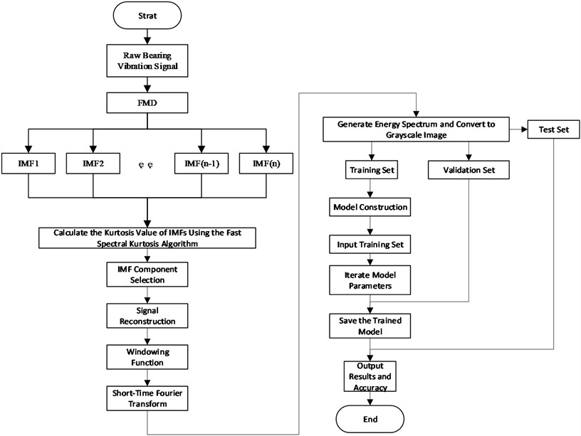
Fig. 1 detailed steps outlined:

1) Signal Decomposition via FMD: The raw vibration signal is decomposed using FMD to extract multiple Intrinsic Mode Function (IMF) components.

2) Target IMF Component Selection: Calculate the spectral kurtosis of each IMF component to quantify its impulsiveness and non-Gaussianity. Identify the maximum kurtosis value and its corresponding characteristic frequency for each IMF. Select IMF components whose characteristic frequencies fall within the original signal’s frequency band as target components.

3) Signal Reconstruction: Reconstruct the filtered IMF components to synthesize a noise-suppressed signal enhanced with fault-related features.

4) Time-Frequency Analysis: Apply Short-Time Fourier Transform (STFT) to the reconstructed signal and compute its energy spectrum to capture transient fault dynamics.

5) Dataset Preparation: Convert the energy spectrum into a grayscale image and partition it into training, validation, and test sets for model development.

6) CNN Model Training: Train the preconfigured CNN model using the training set to learn discriminative fault patterns. Save the optimized model weights after training completion.

7) Hyperparameter Tuning: Evaluate the model’s performance on the validation set to refine hyperparameters (e.g., learning rate, dropout rate). Store the fine-tuned model for subsequent testing.

8) Model Evaluation: Deploy the finalized model on the test set to assess its diagnostic accuracy and generalization capability.

5. Simulation analysis

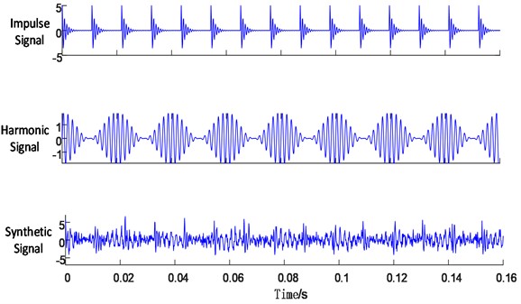
A mixed simulation signal is constructed to evaluate the reasonableness of the proposed algorithm, which consists of a shock signal, a harmonic signal, and non-periodic signal. As demonstrated in Eq. (10):

where $x_3\left(t\right)$ are noise signals with signal-to-noise ratio of 6. Their time domain waveforms are shown in Fig. 2

Fig. 2Time-domain waveforms of the simulated signal and its components

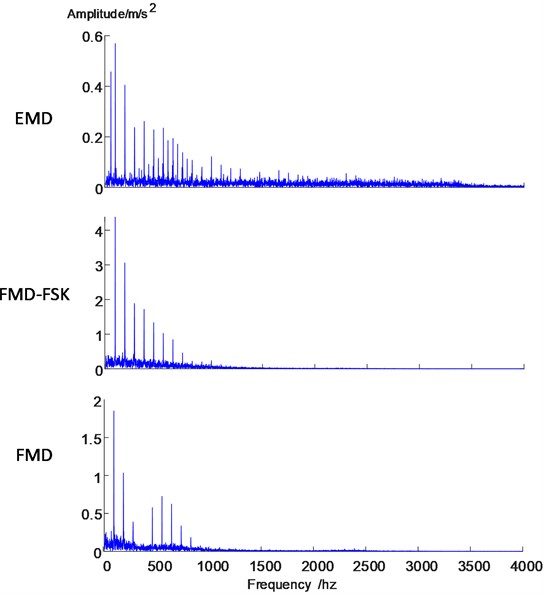
The signal’s modal decomposition is executed utilizing EMD and FMD, respectively, while modal screening and reconstruction are conducted through the FSK method and the conventional correlation coefficient method, respectively. Envelope diagrams for the three methods will be provided to facilitate a comparative analysis of the decomposition and screening effects.

Fig. 3 illustrates that the signal envelope reconstructed through correlation coefficient screening following EMD algorithm decomposition exhibits a greater number of impactful spectral lines, accompanied by numerous trans-frequency sidebands adjacent to the eigenfrequency spectral lines, which lack sufficient clarity for convolutional neural network input. Conversely, after FMD algorithm decomposition and correlation coefficient screening, the reconstructed signal envelope displays more distinct spectral lines; however, the eigenfrequency spectral lines remain inadequately pronounced. Following the decomposition of the FMD algorithm and the application of FSK screening for signal reconstruction, the envelope map exhibits reduced clutter. A notable increase in amplitude signifies a substantial enhancement of fault characteristics, thereby providing a distinct advantage in subsequent image recognition and fault diagnosis.

Fig. 3Envelope diagrams of FMD, FMD-FSK, and EMD

6. Case study

6.2. Digital signal preprocessing

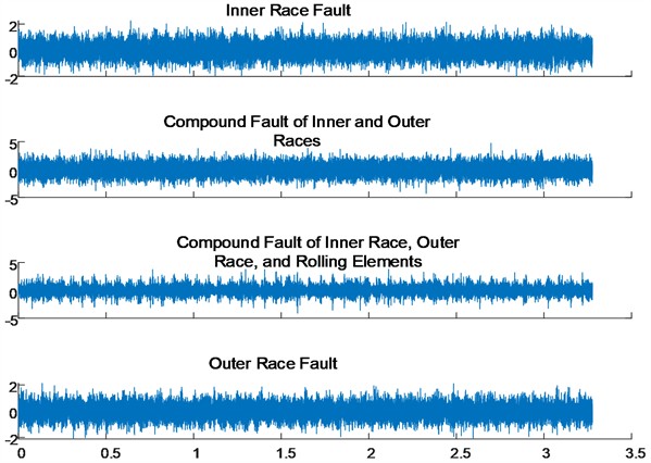
The experiment utilises the segment of the dataset with a collection frequency of 10 kn, encompassing four fault types: inner-race fault, outer-race fault, composite fault of the inner and outer race (IOF), and composite fault involving the inner and outer race along with the rolling elements (IORF). Fig. 5 illustrates the time-domain signal waveforms for each fault type, revealing that composite faults exhibit a higher amplitude compared to single fault types; however, distinguishing them based on waveform characteristics proves challenging.

Fig. 4Experimental platforms [18]

Fig. 5Bearing fault signals

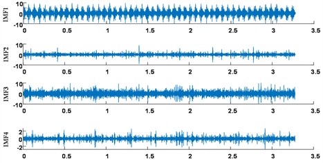
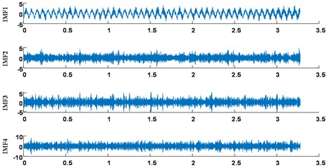
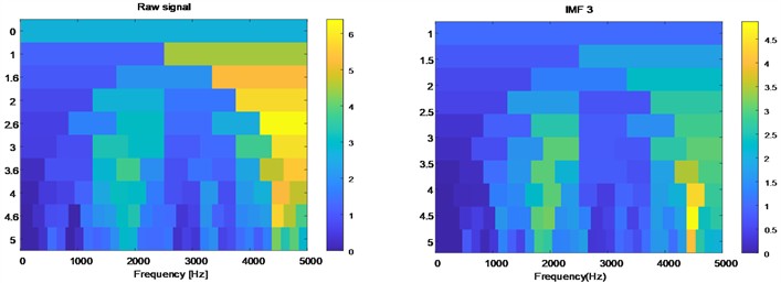
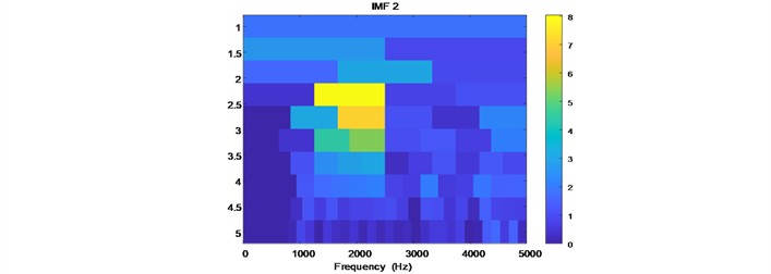
To address the issue, the signal in the dataset is initially dissected utilizing the FMD technique, as illustrated in Fig. 6, which displays the first four IMF components of a defective signal post-FMD decomposition. All four defective signals are subjected to this form of decomposition. Following signal decomposition, it is essential to compute the spectral gradient of both the original signal and each IMF component. The maximum spectral gradient must be identified, and a comparison should be made to ascertain whether the frequency band corresponding to the maximum gradient of each IMF component falls within the band of the maximum gradient of the original signal. This process is illustrated in Fig. 7, which presents the spectral gradient diagrams for the original signal and several IMF components. The maximum gradient of the original signal is 6.4, occurring within the frequency range of 4192 Hz to 5000 Hz. The IMF3 component exhibits a maximum gradient within the interval of 4220 Hz to 4335 Hz, which is situated within the original signal’s maximum gradient range, thus classifying it as an effective component. Conversely, the IMF2 component's target interval does not overlap with that of the original signal and is therefore excluded. The approach is utilized for all vibration signals, and if several valid IMF components exist, the chosen IMF components are then reconstructed.

To enhance the precision of subsequent experiments, the validated and reconstructed signals are converted into spectrograms via the short-time Fourier transform, and these spectrograms are normalized into visual grayscale maps to serve as inputs for the convolutional neural network.

Fig. 6Intrinsic mode function

a) Inner race fault signal

b) Outer race fault signal

Fig. 7Spectral kurtosis diagrams of the raw signal and IMF components

To enhance the accuracy of subsequent experiments, the screened valid signals and reconstructed signals are converted into time-frequency spectrograms using the STFT. The generated spectrograms are then normalized into grayscale images, which serve as standardized inputs to the CNN.

6.4. Results

This experiment classifies bearing failure into four categories: inner ring failure, outer ring failure, composite failure of the inner and outer rings, and composite failure of the inner ring and rolling bodies. This categorization occurs during the generation of the grayscale map through signal preprocessing. Subsequently, 500 randomly selected grayscale maps are allocated into a training set, validation set, and test set, with the training set comprising 70 %, the validation set 10 %, and the test set 20 %.

Fig. 8Spectral kurtosis diagrams of the raw signal and IMF components

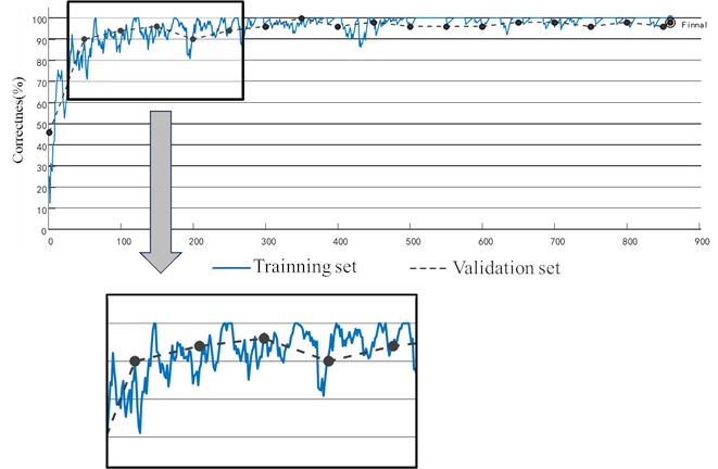
The apparatus utilized for the experiment comprises an 11th Gen Intel(R) Core(TM) i7-11800H processor and an NVIDIA GeForce RTX 3060 Laptop GPU, with a total of 800 iterations scheduled. Fig. 8 illustrates the training outcomes, indicating that the accuracy of the experimental samples ascends to 100 % for the first time at the 90th iteration, while the accuracy of the validation set concurrently achieves 100 % without exhibiting overfitting conditions. The remaining test sets are incorporated into the finalized training model for prediction, with results illustrated in Fig. 9. The horizontal axis represents the predicted fault type, while the vertical axis denotes the actual fault type. The model achieves an average accuracy of 98 %, with a diagnostic accuracy of 100 % for mixed fault types. This demonstrates that the methodology presented in the paper effectively diagnoses composite faults of varying types, accurately identifies the fault signals associated with each type, and subsequently diagnoses the fault signals of different fault types. defects, identifying the attributes of each defect signal.

Fig. 9Model prediction results diagram

6.5. Comparison experiment

This research will employ various methodologies for experimental comparison to validate the superiority of the proposed approach.

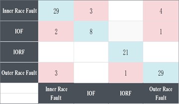
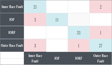
Fig. 10 illustrates that the FMD-FSK-CNN and FMD-CNN exhibit minimal disparity in the convergence speed of the validation set's accuracy. Although the initial accuracy of the validation set is slightly different, the FMD-FSK-CNN method sustains an accuracy of 98 % and achieves 100 % at certain intervals during subsequent iterations. The accuracy of FMD-CNN varies between 90 % and 95 %. As illustrated in Fig. 11(a) and Fig. 11(b), both techniques achieve an accuracy of one hundred percent for composite defects, with minimal error observed in instances of inner and outer ring faults. This comparative experiment demonstrates that fault diagnosis with the FMD approach exhibits superior diagnostic capabilities for composite fault issues, while the accuracy of the enhanced FMD method has been further elevated, along with a notable improvement in stability.

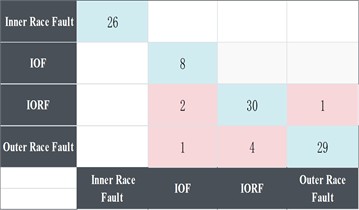
In comparing the FMD-FSK method with the EMD-FSK method, as illustrated in Fig. 10, the EMD algorithm exhibits a smoother curve post-convergence of the validation set; however, its accuracy stabilizes at approximately 90 percent. Furthermore, the confusion matrix in Fig. 11(c) indicates that the EMD method struggles to effectively decompose features when confronted with multiple composite fault scenarios, resulting in a higher incidence of misdiagnosis across various fault types.

The FMD-FSK-CNN method is juxtaposed with the FMD-FSK-BP method. As illustrated in Fig. 11(d), the convergence rate of the BP neural network is markedly inferior to that of the convolutional neural network. Furthermore, the accuracy achieved post-convergence fails to meet expectations, while the validation set accuracy exhibits significant fluctuations. The confusion matrix indicates a substantial number of errors in the model's performance following training, thereby demonstrating the inadequacy of the BP neural network when addressing two-dimensional images.

In comparing the FMD-FSK-CNN method with the VMD-CNN method, as illustrated in Fig. 10, the conventional VMD method exhibits a lower initial accuracy on the validation set compared to the FMD method. Additionally, its convergence rate is slower than that of the FMD-FSK-CNN method. Although it demonstrates strong stability post-convergence, its accuracy is only sustained at 90 %. Fig. 11(e) illustrates that the conventional VMD approach remains inadequate for the composite fault issue, exhibiting a higher rate of misdiagnosis and demonstrating marginally inferior overall accuracy compared to the FMD-FSK-CNN method.

Fig. 10Correctness of the validation set for each method

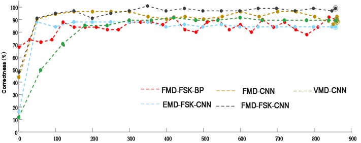
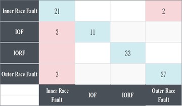
Fig. 11Confusion matrix for each method

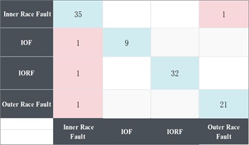
a) Confusion matrix for FMD-CNN accuracy`

b) Confusion matrix for FMD-FSK-CNN accuracy

c) Confusion matrix for EMD-FSK-CNN accuracy

d) Confusion matrix for FMD-FSK-BP accuracy

e) Confusion matrix for VMD-CNN accuracy

Table 2Test set accuracy for each method

Usage	Correctness / %
FMD-FSK-CNN	96.2 %
FMD-CNN	92 %
EMD-FSK-CNN	86.1 %
FMD-FSK-BP	90.0 %
VMD-CNN	92.1 %

7. Conclusions

The article introduces the FMD-FSK-CNN approach for bearing failure diagnosis, validated through the integration of the FMD algorithm with FSK and the application of convolutional neural networks.

The FMD algorithm and FSK, when combined, effectively screen out components with strong features, further enhancing the processing capability for composite fault problems and strengthening the noise immunity capability. This method is more applicable and can better distinguish the fault features in a strong noise environment, while also amplifying the feature signals to make them serve as high-quality CNN inputs. In comparison to traditional EMD and other methods. Information.

The integration of CNN and FMD-FSK methods and their comparison experiments have resulted in an 8 % increase in the accuracy of the verification set, which can more accurately identify the type of each composite fault. This demonstrates the method's intelligence, superiority, and effectiveness.

Future Outlook: Nevertheless, the method described in this paper still necessitates the manual adjustment of certain parameters in the context of FMD. The modification of this parameter has a significant impact on the effect's functionality and is contingent upon the user's experience. There is no more consistent evaluation standard, necessitating further optimization of the FMD method to meet the demand. However, the screening of IMF components decomposed by FMD using the FSK technique requires a longer time than the EMD method, necessitating further optimization.