Abstract
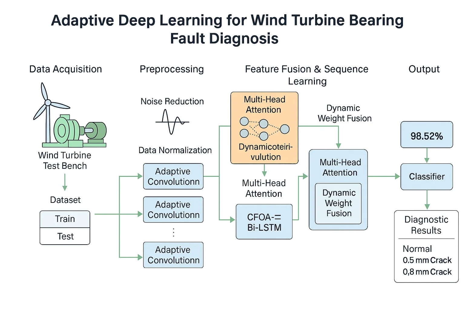
In response to the problem of difficulty in extracting fault features of rolling bearings in wind turbine transmission systems under complex working conditions, which limits the accuracy of fault diagnosis. This article proposes an Adaptive Deep Learning based Rolling Bearing Fault Diagnosis Method (ADLM). Introducing dynamic convolution into Convolutional Neural Networks (CNNs) can adaptively capture data features; At the same time, the fishing optimization algorithm (CFOA) was used to optimize the hyperparameters of the bidirectional long short-term memory network (BiLSTM), and the CFOA-BiLSTM network was constructed to fully leverage its advantages in time series analysis. The specific implementation steps are as follows: first, preprocess the collected vibration signals and divide the processed dataset into a training set and a testing set; Then, parallel adaptive convolutional neural networks (ACNN) are used to process the training set and extract spatial domain local features from the vibration signal; Then, the features extracted from the two branches are weighted and fused through a dynamic weight adjustment mechanism, and the fused features are input into the CFOA-BiLSTM network to further capture the time-dependent features of the signal; Finally, the extracted features are input into the classifier to complete model training, and the model performance is evaluated using a test set. Experimental verification shows that on the dataset of Southeast University, the diagnostic accuracy of the ADLM model reached 98.52 %, demonstrating good reliability, robustness, and superiority in the diagnosis of rolling bearing faults.
Highlights
- Adaptive feature extraction: Introduced a parallel Adaptive Convolutional Neural Network (ACNN) with dynamic convolution to capture multi-scale spatial features from bearing vibration signals.
- Optimized sequence modeling: Applied Catch Fish Optimization Algorithm (CFOA) to tune BiLSTM hyperparameters, enhancing time-series feature learning and improving convergence.
- Dynamic feature fusion: Designed a dynamic weight adjustment mechanism using multi-head attention to adaptively integrate multi-branch ACNN outputs.
- Superior diagnostic performance: Achieved 98.52% accuracy on Southeast University wind turbine bearing dataset, outperforming ANN, TCN, and MSCNN by over 58%.
- Robustness under complex conditions: Ablation experiments confirmed the critical contribution of each module to stability and accuracy in noisy and variable-speed environments.
1. Introduction
Rolling bearings play a key role in wind turbines. Their performance and reliability are crucial to ensuring the stable operation of the entire wind turbine. Rolling bearings operate in harsh working environments and are subject to complex load changes, making them prone to various faults such as wear, cracks, and spalling [1]. If the fault is not discovered and handled in a timely manner, the equipment may shut down, production efficiency may be reduced, and even serious safety accidents may occur [2-3]. Therefore, in order to ensure the safe operation of wind turbines, it is necessary to conduct research on intelligent monitoring and diagnosis of rolling bearings [4-5].
With the advancement of monitoring technology and the increasing complexity of mechanical equipment structures, deep learning technology has attracted attention for its ability to automatically extract deep fault features. It eliminates the need to rely on traditional expert systems. Its multi-level structure gives it powerful data fitting and processing capabilities, and it can efficiently process and analyze complex data sets. Wang et al. [6] developed a fault diagnosis technology that combines short-time Fourier transform with convolutional neural network. This technology effectively utilizes the time-frequency characteristics of the signal and enhances the accuracy and efficiency of fault diagnosis through the efficient feature extraction capability of the deep learning model. Zhao et al. [7] proposed an improved CNN model for rolling bearing fault diagnosis under changing working conditions. This method can effectively capture the key features in sample data even in a high noise environment by distributing feature extraction tasks in convolutional layers of different scales. Wang et al. [8] proposed a collaborative intelligent fault detection method based on swarm intelligent optimization entropy (SIOE) and extreme gradient boosting (XGBoost), which significantly improves the fault diagnosis accuracy of rotating machinery through adaptive parameter optimization and dynamic feature extraction. In order to solve the problem of complex fault diagnosis of planetary gearboxes, Sun et al. [9] proposed an improved particle swarm optimization variational mode decomposition (IPVMD) and an improved convolutional neural network (I-CNN). Wang et al. [10] proposed a small-sample fault diagnosis method based on multi-scale perception multi-level feature fusion image quadrant entropy, which achieves more than 98.1 % accuracy with only 5 training samples by signal image-based transformation and multi-level feature extraction combined with optimized support vector machine classifier. Hu et al. [11] studied the rolling bearing fault diagnosis method based on target detection theory. They took the rolling bearing of printing equipment as the research object and explored the rolling bearing fault diagnosis method based on target detection theory from the two aspects of time domain and time-frequency domain. The performance of the method was verified through multiple experiments. Wang et al. [12] proposed a generalized fault diagnosis framework based on multi-scale phase entropy and time-shift decomposition, combining scatterplot regional probabilistic features and twinned support vector machine classifiers to achieve over 99.5 % high accuracy fault identification with multiple metrics with a small number of training samples.
Rolling bearings, due to their complex operating structure, drastically changing loads and extremely harsh working environment, make the collected signals very complex and show nonlinear characteristics. This increases the complexity of manually selecting appropriate feature indicators for signal processing. Simple fault diagnosis models cannot meet the changing working conditions, while overly complex algorithm models may affect the diagnosis efficiency and reduce the versatility.
In response to the above challenges, this paper proposes a rolling bearing fault diagnosis method based on adaptive deep learning. The main innovative points are as follows:
(1) In this paper, a dynamic convolution mechanism is introduced on the basis of traditional CNN, and an adaptive convolutional neural network (ACNN) is constructed, which is capable of dynamically adjusting the parameters of the convolution kernel according to the feature distributions of the input data, so as to capture the local spatial features of the bearing vibration signals more effectively. Further, a parallel ACNN structure is designed to realize the extraction of multi-level features of the signal through multi-scale convolution operation, which enhances the models ability to perceive complex fault features.
(2) In order to give full play to the advantages of BiLSTM in time series modeling, this paper adopts CFOA to optimize its key hyperparameters, and constructs the CFOA-BiLSTM network, which improves the convergence speed and generalization performance of the model.
(3) A dynamic weight fusion mechanism is designed to adaptively weight and integrate the spatial features extracted from multiple branches of parallel ACNN. This mechanism can automatically assign weights according to the discriminative strength of fault features, and enhance the extraction efficiency of fault-sensitive features such as shock pulse and frequency modulation.
This method first preprocesses the collected vibration signal, including outlier removal and duplicate value integration, and divides the preprocessed data set into a training set and a test set; then the training set is input into two parallel ACNN branches, and ACNN uses its ability to extract local features in the spatial domain from the vibration signal; the features extracted by the two branches are weighted and fused, and then input into the CFOA-BiLSTM network, and BiLSTM uses its advantages in time series analysis to capture the time-dependent characteristics of the signal; the combination of the two feature extraction methods enables the model to understand the fault information in the vibration signal more comprehensively, and then the final extracted features are input into the classifier to complete the training of the entire model; finally, the test set is input to evaluate the performance of the entire model. After comparative testing, the effectiveness of this method is verified.
2. Basic theory
2.1. Adaptive convolutional neural network (ACNN)
Convolutional Neural Networks (CNN) is a widely used network architecture in the field of deep learning. Due to its weight sharing mechanism [13], it can play its own advantages when processing high-dimensional data information. CNN extracts features from the original signal by multiple convolutional layers and pooling layers, maps the extracted features to the hidden feature space, and then uses the fully connected layer to further extract the features. The detailed structure is shown in Fig. 1.
Fig. 1Convolutional neural network structure diagram

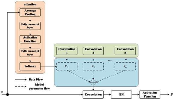
(1) Dynamic convolution. Traditional convolution limits the number of convolutional layers and channels of CNN due to the low computational budget, which will reduce the model performance, so dynamic convolution was proposed [14]. It dynamically aggregates multiple parallel convolution kernels based on attention. Attention dynamically adjusts the weight of each convolution kernel according to the input, thereby generating adaptive dynamic convolution. The attention superimposes the convolution kernel in a nonlinear way to make it have stronger representation ability. Its structure diagram is shown in Fig. 2, and the mathematical formula is as follows:
where: is the attention weight of the th linear function ; the aggregation weight and the deviation are functions of the input with the same attention.
(2) Activation layer. After each convolutional layer, an activation layer (nonlinear layer) is usually applied [15] to enhance the nonlinear expression ability of the signal. The most widely used is the rectified linear unit (ReLU), which can speed up convergence and overcome the vanishing gradient. The mathematical expression of the ReLU activation function is as follows:
Fig. 2Dynamic convolution structure diagram
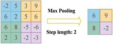
(3) Pooling layer. Common pooling layers include maximum pooling and average pooling. Their main purpose is to effectively reduce the dimension of the feature space, thereby reducing the number of parameters in the network as a whole, improving computational efficiency and enhancing the generalization ability of the model. The reason why the pooling layer is introduced after the convolution layer is that there are many convolution kernels in the convolution layer. After the convolution operation with weight sharing, the feature dimension of the output increases, which leads to the expansion of the network parameter scale and increases the computational complexity of subsequent feature extraction. The pooling layer represents the information of the area by selecting the maximum value or average value in a window of a specific size, thereby achieving effective dimensionality reduction of the features. Maximum pooling selects the maximum value in the window as the output, which helps to highlight the most important features and is invariant to small position changes. Average pooling calculates the average value of all values in the window, which helps to smooth the feature response and reduce the impact of noise. Maximum pooling is widely used in CNN design because it can retain the most significant features and enhance the invariance of features. Its structure diagram is shown in Fig. 3, and the function expression is as follows:
where: represents the th pooling value at the th position in the th layer output mapping, represents the local input feature of the th pooling process, and is the width of the pooling window. The calculation process can be represented by the following diagram.
Fig. 3Schematic diagram of maximum pooling
(4) Fully connected layer. In the feature extraction process, the convolution layer and pooling layer mainly capture the local key features of the data, while the fully connected layer is responsible for comprehensive processing and analysis of the local information. Finally, the classification result is obtained by using the above extracted features for prediction and classification. The main function of the fully connected layer is to map the previously extracted features to the final category. Its calculation process can be expressed by the following formula:
where: represents the th layer of the network, is the input of the st fully connected layer, is the output of the th fully connected layer, is the weight matrix, is the bias term, and is the classification function.
The softmax function is used as the activation function of the fully connected layer. Its function is to convert the output of multiple neurons into the (0, 1) interval to handle multi-classification problems. Its formula is as follows:
where: is the logical input of the function layer, which produces a -dimensional probability distribution. The function converts the output of the last layer of the network into a probability value that sums to 1 through a specific mathematical formula. The category of the sample is determined by the label with the highest probability value.
2.2. Dynamic weight adjustment mechanism
When fusing features, a multi-head attention mechanism module is used to calculate the weight of each feature for weighted fusion. In dynamic weight adjustment, the multi-head attention mechanism can be used to more finely adjust the weights of different features, thereby improving the expressiveness and adaptability of the model. The multi-head attention mechanism is the core technology of the Transformer architecture, which is implemented through multiple parallel self-attention modules. Each attention head operates in an independent subspace, focusing on capturing information of different dimensions in the sequence data, allowing the model to focus on multiple key features at the same time. These output results from different heads are merged and integrated through a linear transformation layer to finally generate the output of the model. The entire calculation process is as follows:
First, the features extracted by ACNN are concatenated into a joint feature:
In the formula, is the concatenated feature, and and are the features extracted by two parallel branches respectively.
Map the concatenated features to multiple subspaces through linear transformation:
where: , , are learnable weight matrices, , , are query, key, and value, respectively.
Calculate the attention score in each attention head:
where: is the dimension of the key and the softmax function is used to normalize the attention score.
Concatenate the outputs of multiple attention heads:
where: is the number of attention heads and is the learnable weight matrix.
The dynamic weights are calculated using the output of the multi-head attention mechanism:
where, and are the dynamic weights of the features of the two ACNN branches.
Weighted fusion of the features of the two branches of ACNN:
where: is the fused feature.
2.3. Overview of the BiLSTM Network Structure
(1) Overview of the LSTM Network Structure. Recurrent Neural Network (RNN) is a kind of deep learning model, which is specially designed for sequence data processing. However, when it is used to process long sequence data, there will be problems of gradient disappearance or gradient explosion, which limit the application ability of RNN in the fields of time series prediction, language model and speech recognition. Therefore, Long Short-Term Memory network (LSTM) was proposed.
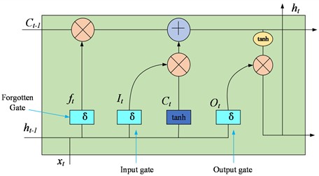
LSTM is an improved version of the RNN architecture that replaces the normal hidden units in RNN by introducing three gating mechanisms and memory units that enable it to capture information delayed over long time intervals and time sequences. The three gating mechanisms are forgetting gate, input gate and output gate. The structure of LSTM is shown in Fig. 4.
Fig. 4Neural Structure of LSTM Network
The memory cell is the core of LSTM, storing the long-term state information in the sequence. By controlling the inflow and outflow of information as well as the update of the internal state, it enables the network to selectively remember or forget certain information segments, thereby solving the problem of long-term dependency.
The forgetting gate decides which information needs to be retained and which needs to be forgotten based on the hidden state of the previous moment and the current input. The decision-making process is based on a sigmoid activation function that determines the proportion of each state to be retained, thus dynamically adjusting the content of the memory cells to ensure that the network focuses on remembering the information that is useful for subsequent predictions. the sigmoid function gives an output value between (0, 1), which determines how much of the previous moment's information is retained. The formula for the forgetting gate is as follows:
where: is the weight of the forget gate, is the bias, and is the sigmoid activation function.
The input gate also determines what input information of the current moment can be stored in the memory unit based on the hidden state of the previous moment and the current input. It is achieved through a combination of a sigmoid activation function, where the sigmoid activation function represents the importance of the information, and a activation function, where the tanh function is the concrete content that generates the new information. The calculation process of the input gate is as follows:
Input candidate vector: first, the input gate generates a new set of candidate values, which are learned through the network and used to update the cell state. Candidate values are calculated by the following formula:
Input modulation vector: Used to determine which candidate values will be added to the cell state. This modulation vector is given by the following formula:
Update the cell state: Finally, the update of the cell state at the time step is determined by the forgetting gate output , the input candidate vector , and the input modulation vector :
The output gate decides which information to output as the hidden state for the current time step, based on the updated memory cell state and the current input. It is composed of a simoid activation function and a point-by-point product operation, where the sigmoid activation function is used to determine which information should be forgotten when passing to the subsequent time step, i.e., to determine which information is no longer current or relevant, and the point-by-point product operation is used to determine the information that is ultimately retained and passed to the next time step. Based on this the final output information is generated which will be passed to the LSTM unit at the next time step. The formula for the output gate is as follows:
(2) Overview of BiLSTM network structure. LSTM is capable of retaining and remembering the more critical historical data, but it is unable to fully utilise the hidden data of the subsequent neurons, preventing it from capturing future information, which may lead to incomplete information about the final state, limiting its feature extraction ability, which in turn may affect the accuracy of model prediction and classification. In order to capture future data more effectively, Bidirectional Long Short-Term Memory (BiLSTM) has been proposed.
BiLSTM is a network architecture that combines two independent LSTMs, where one LSTM deals with the forward information of sequence information (from the past to the future), and the other LSTM network deals with the reverse information of sequence information (from never to the past). This enables a comprehensive capture of sequence information, allowing BiLSTM to take into account both past and future contextual information for a more detailed and in-depth understanding of each time point in the sequence. The architecture of BiLSTM is shown in Fig. 5.
Fig. 5BiLSTM network structure diagram
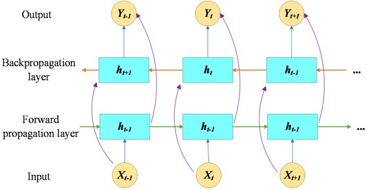
Each LSTM has its own internal state, as well as its own cellular and hidden states, and its own weight matrix and bias terms. So, a BiLSTM network contains two complete sets of LSTM parameters, which makes it capable of capturing richer features in a sequence. It also makes BiLSTM particularly suitable for tasks involving sequence data, such as natural language processing, where textual information can be extracted and utilised in a more comprehensive way, leading to excellent performance in applications such as sentiment analysis, text classification and machine translation.
The forward and backward mathematical expressions of BiLSTM are as follows:
where: denotes the computation result of the LSTM hidden layer; denotes the input data at time step ; denotes the input weight of the LSTM; denotes the weight at time step ; denotes the bias term of the LSTM layer; and represents the activation function.
The calculation formula of the output layer is as follows:
where: denotes the output of the final output layer, which is calculated by superimposing the output values of the two hidden layers at each time step.
2.4. Fishing optimisation algorithms
CFOA is a meta-heuristic optimisation algorithm proposed by Jia et al. [16], which simulates the process of fishing in water by rural fishermen. During the fishermen’s search for fish nests, they actively disturb the water along the way, causing turbidity, which is conducive to fishing. Fishermen co-operate with each other and use nets to encircle potential fish populations, preventing fish from escaping and thus increasing the overall catch rate. All the fishermen drive the fish to a common location, forming a closed circle to maximise the aggregation of all the fish, which ultimately leads to catching the most fish. The process is divided into initialisation, exploration phase and exploitation phase. While in the exploration phase the choice of whether to catch independently or cooperatively as a group is made based on the number of fish.
1. Initialization.
The initialization formula is:
where, is the position of the th fisher in the th dimension, and are the upper and lower bounds of the t dimension, and is a random number between (0, 1).
2. Exploration stage ( 0.5).
Fish are most abundant and catch rates are highest at the very beginning of the fishery, but as fishermen's catch gradually decreases, this leads to a decline in catch rates. Transitions in this model are simulated using the catch rate parameter, denoted as a:
where, is the current number of assessments and is the maximum number of assessments.
Fishermen are free to choose either independent search or group capture, but when the capture rate is high, fishermen’s capture strategy tends to favor the independent search method, and when the capture rate decreases, fishermen shift to the group capture method, which we simulate using the random number (0, 1). Independent search is chosen when , and group capture is chosen when . is the probability, a random number between (0, 1).
(1) Independent search ().
Fishermen adjust the direction and location of their own exploration based on the catches of others. Focuses on localized exploration if the catch situation at their location is similar to the reference catch situation. If the reference catch situation was favorable, they continued to search in that direction. In cases where the individual capture situation was favorable, they conducted a reverse search. The update formula is as follows:
where, is the empirical analysis value obtained by the fisherman with any th ( 1, 2,...,, ) fishermen as the reference object, which takes the range of (–1, 1). and are the worst and best fitness values after the complete position update, respectively. denotes the number of iterations of the fishermen’s position. and represents the position of the th fisherman in the th dimension and after and iterations. is a random number between (0, 1). is the Euclidean distance between the individual and the reference. is a -dimensional random unit vector. Based on the empirical analysis, the main direction of travel (with the direction from the fisherman to the reference individual as the positive direction) and the distance are determined. The exploration range also varies with the absolute value of and the number of currently evaluated , with less than or equal to .
(2) Group fishing ().
Fishers expand their fishing capacity and randomly form groups of 3-4 people who cooperate with each other to encircle suspected sites. As fish continue to be caught and people gradually gather, the degree of deviation in fishermen’s movement decreases. The area is explored more accurately by utilizing the unique movement capabilities of each individual. The modeling and formulas are as follows:
where, is a group of 3-4 individuals whose positions are not updated. is the target point of the group envelope, i.e., the reddish-orange point in the figure below. and denote the positions of the th fisher in group in dimension after and updates. is the speed at which the fisher approaches the center, which varies from individual to individual and takes the value in the range of (0, 1). is the offset of the movement, which takes the value in the range of (–1, 1), which decreases with the increase of .
3. Exploitation phase (0.5).
After the above stage, some fish escape without being caught by the fishermen. Therefore, in this stage, the distribution of fishermen is as follows: centered on the fish stock, the degree of aggregation from the middle to the periphery is gradually sparse, and the range of distribution outward is gradually reduced. The fishermen in the center catch the school while the fishermen in the periphery catch the escaped fish. Fishermen fish strategically in a concerted effort to increase catch rates. A Gaussian distribution is used to model this distribution, updating the formula as follows:
where, is a Gaussian distribution function with an overall variance σ increasing from 0-1 with the number of evaluations. is the position of the th fisher after updates. is a matrix of the mean values of each dimension of the fisher center. is the global optimal position, and is a random number with value {1, 2 or 3}.
CFOA initializes a series of key parameters in terms of parameter setting, the population size is set to 50, this number is determined after several experimental tests, taking into account the computational cost and algorithm performance, which can ensure that the algorithm effectively explores the solution space while maintaining a reasonable computational burden. The maximum number of iterations is set to 200 to ensure that the algorithm has enough iterations to converge to a better solution. The initial value of the capture rate parameter is set to 0.6, and its value will be dynamically adjusted based on the ratio of the current FFs to during the iteration process of the algorithm to balance the algorithm's exploratory and exploitative capabilities, with the algorithm more inclined to explore globally in the first half of the stage () and focusing on local search in the second half of the stage ().
2.5. Hyperparameter optimization of BiLSTMs
1. Hyperparameter optimization range.
Several key hyperparameters of the BiLSTM model are optimized using CFOA, specifically involving the following hyperparameters and their corresponding optimization ranges:
Learning rate: the learning rate has a key impact on the convergence speed and performance of the model. In this study, we set its optimization range to [0.0001, 0.1]. Too small a value will result in extremely slow model training, which may not converge to a better solution for a long time; while too large a value may cause the model to miss the optimal solution during the training process, resulting in failure to converge or even divergence. Optimization within this range is aimed at exploring a learning rate that ensures both training efficiency and model convergence to good performance.
Number of hidden layer nodes: the number of hidden layer nodes determines the learning ability and complexity of the BiLSTM model. We set its optimization range to [32, 256]. If the number of nodes is too small, the model may not be able to fully learn the complex features and patterns in the data, resulting in underfitting; conversely, if the number of nodes is too large, the model may learn too much noise and details, resulting in overfitting, and at the same time, increase the computational cost and training time. By searching for the optimal number of nodes in this range, it is expected to construct a model with appropriate complexity to balance the learning ability and generalization performance.
Dropout rate: as an effective means to prevent overfitting, the rate setting of Dropout has a significant impact on the model performance. We set the optimization range as [0.2, 0.8]. When the Dropout rate is too low, it is difficult for the model to effectively avoid overfitting; while when the Dropout rate is too high, neurons may be excessively discarded, leading to a decrease in the model’s learning ability and underfitting. Optimizing the Dropout rate within this range helps to find a balance that can suppress overfitting while maintaining the model learning ability.
2. Optimization objective function.
The optimization objective function of the CFOA algorithm is constructed based on the classification accuracy. In our research task, the classification accuracy rate can intuitively and effectively measure the ability of BiLSTM model to correctly classify various types of samples. Specifically, the optimization objective function is to maximize the classification accuracy, i.e.:
where, is the true case, the number of instances that the model correctly predicts as positive classes; is the true negative case, the number of instances that the model correctly predicts as negative classes; is the false positive case, the number of instances of negative classes that the model incorrectly predicts as positive classes; and is the false negative case, the number of instances of positive classes that the model incorrectly predicts as negative classes.
This metric is used as the optimization objective because we expect to find a set of optimal BiLSTM hyperparameters through the CFOA algorithm, so that the model can achieve as high an accuracy as possible when classifying the target data, thus improving the overall performance and reliability of the model. In the process of model training and CFOA optimization, each iteration evaluates the advantages and disadvantages of the model based on the classification accuracy of the current hyperparameter combination on the validation set, and guides the CFOA algorithm in updating and adjusting the hyperparameters until it finds the combination of hyperparameters with the highest classification accuracy.
3. Introduction to the model
3.1. The model in this paper
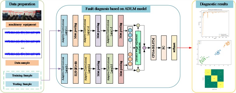
In this paper, an ADLM model is built based on ACNN and CFOA-BiLSTM. The core of the method is to use the powerful feature extraction capability of ACNN and the advantage of CFOA-BiLSTM in sequence information to extract effective features from the vibration signal to complete the fault diagnosis classification of rolling bearings. Its model structure is shown in Fig. 6.
In this method, the whole process includes five steps: signal acquisition, data preprocessing, model construction and result output. Firstly, the vibration signal data is obtained through the sensor installed in the transmission part of the wind turbine; Secondly, the collected vibration signals are preprocessed, including outlier elimination and repeated value integration, and the preprocessed data set is divided into training set and test set. Then the training set is input into two parallel ACNN branches, and ACNN uses its ability to extract local features in spatial domain from vibration signals. The features extracted from the two branches are weighted and fused using a dynamic weight adjustment mechanism, and then fed into the CFOA-BiLSTM network, which captures the time-dependent features of the signals with its advantage in time-series analysis; the combination of the two feature extraction methods enables the model to understand the fault information in the vibration signals in a more comprehensive way, and then the extracted features are fed into the classifier to complete the model. The final extracted features are then fed into the classifier to complete the training of the whole model; finally, they are fed into the test set to evaluate the performance of the whole model. The detailed flow of the rolling bearing fault diagnosis method based on ADLM is shown in Fig. 7.
Fig. 6ADLM model diagram

Fig. 7ADLM-based fault diagnosis flowchart
3.2. Data acquisition
In this study, the wind turbine drive train simulation test bed of Southeast University was borrowed, which is capable of reproducing the wind turbine drive train to ensure the reliability of the collected data. The test bed is shown in Fig. 8.
This experimental bench collects the vibration signals generated by rolling bearings in actual operation by simulating the operation of the transmission system of wind turbines. It mainly consists of several components such as motor, sensor, coupling, rolling bearing, gearbox and main shaft. In addition, the experimental rig is equipped with two different gearboxes, a planetary gearbox and a cylindrical gearbox, to reproduce the wind turbine speed increase mechanism. In order to capture and analyse the vibration signals during the experiment, the experimental bench also integrates an advanced signal acquisition and analysis system. These components work together to provide an experimental environment capable of simulating the rolling bearing behavior of wind turbines in various operating states.
The sensor used to collect vibration signals is acceleration sensor. Because the frequency response range of acceleration flow sensor is wider, it is more sensitive to the vibration signal changes caused by impact than speed sensor and eddy current sensor. The model of acceleration sensor used in the test is MHS188U. The contact between the sensor and the bearing is smoothed with an abrasive disk, and then the sensor is pressed and adsorbed on the bearing seat using a magnetic holder to guarantee the accuracy of the signal measurement. At the same time, in order to realize the whole cycle sampling of rotational speed, a set of photoelectric sensors is installed on the rotating shaft of the test bench for keying signal acquisition, and the pulse signals of the photoelectric sensors are triggered by the reflective strips installed on the rotating shaft. The EVM-8 vibration data collector developed by the National Engineering Center for Thermal Power Unit Vibration of Southeast University is used. The device includes an embedded system kernel, a high sampling rate high-precision A/D module, an adaptive amplification circuit, and an automatic tracking anti-mixing filter based on CPLD, which is capable of realizing automatic tracking of the signal frequency.
The data set is divided into 80 % for training and 20 % for testing, covering three conditions under one operating condition, namely, bearing normal condition (marked as 0), inner ring crack of 0.5 mm (marked as 1) and inner ring crack of 0.8 mm (marked as 2).
Fig. 8Wind turbine drive train simulation test bench

a) Wind power transmission system simulation test bench physical picture

b) Schematic diagram of wind power transmission system simulation test bench
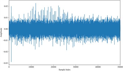
Fig. 9 shows the vibration signals of normal bearing, 0.5 mm and 0.8 mm cracked faulty bearing under the working condition of 40 r/min. As can be seen from the figure, the normal state waveform is smooth, the frequency component is dominated by the rotational fundamental frequency of the bearing, and there is no abnormal shock signal.0.5mm crack state waveform begins to appear in the periodic weak shock pulse, corresponding to the vibration characteristics of the crack and the raceway contact.0.8mm crack state shock pulse amplitude increases significantly, and the high harmonic energy in the frequency component is enhanced, which reflects the vibration aggravation caused by the expansion of the crack.
3.3. Data preprocessing
Data preprocessing can improve data quality, highlight fault characteristics, and facilitate further analysis.
Fig. 9Rolling bearing vibration signal waveforms
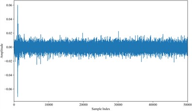
a) Normal rolling bearing signal waveform
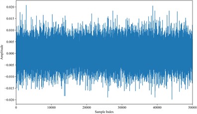
b) 0.5 mm crack rolling bearing signal waveform
c) 0.8 mm crack rolling bearing signal waveform
(1) Noise reduction processing.
As the data set obtained through the acceleration sensor acquisition is not only the useful vibration signal, there are other noises that cause interference, so it is necessary to reduce the noise processing of the collected data. The core of this method lies in combining previous estimation information with current observation data to optimize the estimation of the system's state at the current time point. Due to the dual effects of process noise and measurement noise on actual measurement values, there is a deviation between the predicted output and the actual value. The Kalman filter calculates the Kalman gain by continuously updating the covariance of the system state estimation, combining the filtering error covariance of the previous time and the prediction error covariance of the current time. In the continuous filtering process of the system state, new measurement data is introduced at each step to provide additional information. The discrete form of the Kalman filter linear state equation is as follows:
where: and represent the state vectors at the th and st moments, respectively; is the system noise vector; is the system input; is the system output, which is the observation; is the measurement noise vector; is the state transfer matrix; is the input matrix; is the output matrix. The Kalman filter updates the state estimates in real time and the update process follows the following equation:
where: denotes the state estimate when the observation at moment is not considered, i.e., the a priori state estimate at moment k; is the state estimate obtained after utilizing the observation at moment , i.e., the a posteriori state estimate at moment ; is the a priori estimation error covariance matrix; and is the a posteriori estimation error covariance matrix.
(2) Abnormal data analysis and processing.
During the use of wind turbines, unstable factors such as the external environment or vibration may interfere with data collection, leading to significant anomalies in the data, such as missing data or all-zero data. This type of abnormal data may lead to misleading anomaly detection and condition assessment, which in turn may cause significant errors in the results. Therefore, the collected data need to be cleaned and processed to guarantee the accuracy of rolling bearing condition assessment and its fault diagnosis. Anomalous data usually refers to data that is significantly different from the normal operating condition of a wind turbine, with possible causes including sensor failures, data transmission errors, or uncertainties such as extreme changes in wind speed (too high or too low).
To reduce the impact of abnormal data on rolling bearing fault diagnosis and status assessment, it is necessary to handle these data appropriately to ensure that monitoring parameters can accurately reflect the actual operating conditions of the unit during operation. For unreasonable or stagnant accumulated data points, they need to be directly deleted based on the wind power generation curve. For missing data, it is necessary to decide whether to delete or fill in based on the size of the missing data. Standardization is a commonly used technique in data preprocessing, whose main purpose is to convert data of different dimensions, units, and scales to a unified standard scale. Through standardization processing, differences between data can be eliminated, internal relationships between data can be better displayed, accuracy of data analysis and stability of model establishment can be improved, while model performance can be enhanced and its training process can be accelerated. In this experiment, the maximum minimum normalization technique is applied to standardize the data in order to map the original data to the range of [0, 1].
4. Experimental section
4.1. Comparative experiment
In order to verify the superiority of ADLM in diagnosing and classifying rolling bearing faults under complex working conditions, other mainstream fault diagnosis models were selected for comparison, mainly including the following four types:
(1) This article presents the ADLM model.
(2) Traditional Machine Learning Methods: Artificial Neural Networks(ANN), the hidden layer is a 2-layer fully connected layer with 64 nodes in the first layer and 32 nodes in the second layer, both of which use the ReLU activation function; the number of nodes in the output layer is 3 (corresponding to the three types of states: normal, 0.5-mm crack, and 0.8-mm crack).
(3) Temporal Convolutional Network(TCN), a 3-layer causal convolution is used, with the number of filters in each layer being 32, 64, and 128, respectively, and the size of the convolution kernel is 3 for all of them, and the expansion factors are 1, 2, and 4 in order to capture the multi-scale temporal features, and the ReLU activation function is used after each layer of convolution with the addition of a Batch Normalization layer to accelerate convergence, and a global average pooling is received to the fully-connected layer with the number of nodes being 3.
(4) Multi-scale convolutional neural network (MSCNN), branch 1 uses a 1×1 convolution kernel (capturing local features) with a number of filters of 32 and an activation function ReLU, branch 2 uses a 3×3 convolution kernel (capturing medium-scale features) with a number of filters of 64 and an activation function ReLU, and branch 3 uses a 5×5 convolution kernel (capturing global features) with a number of filters of 128 and an activation function ReLU.
During model training, the learning rate, mini-batch, and training batch were set consistently for each model. The optimizer was the Adam optimizer with a learning rate of 0.0001, the number of training rounds was 50, and the mini-batch size was set to 32. In order to reduce the effect of randomness, each trial was conducted three times. The evaluation criteria are diagnostic accuracy, F1 score, precision, and recall. Diagnostic accuracy is the ratio of correctly diagnosed samples to the total number of samples, which reflects the overall performance of the evaluation method; F1 score reflects the performance of the evaluation method in each category; precision reflects the “accuracy” of the model in predicting the labels of the positive categories; and recall reflects the ability of the model to identify all the samples in the positive categories, i.e., the proportion of the model finding all the samples that are actually positive cases. The recall rate reflects the model's ability to identify all positive samples, i.e. the proportion of actual positive samples identified by the model. The results are shown in Fig. 10 and Table 1.
Fig. 10Comparison of the accuracy of the models
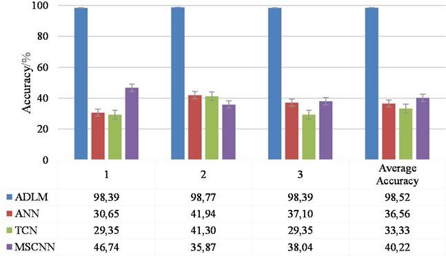
Table 1Results of the rubric for each model
Model | Average F1 score / % | Average precision / % | Average recall / % |
ADLM | 98.51±0.18 | 98.56±0.15 | 98.52±0.18 |
ANN | 36.33±4.51 | 38.37±6.20 | 36.56±4.62 |
TCN | 17.84±4.60 | 12.10±3.60 | 33.33±5.63 |
MSCNN | 20.04±0.83 | 25.51±17.09 | 40.22±4.70 |
As shown in Fig. 10 and Table 1, the method proposed in this paper significantly outperforms the other three models in terms of accuracy, F1 score, precision and recall, and the performance of ANN, TCN, and MSCNN are all under 40 %, except for MSCNN, which has an average accuracy and an average recall just over 40 %. In contrast, the diagnostic accuracy of this paper’s method increases significantly, achieving 61.96 %, 65.19 %, and 58.30 % increases relative to the comparative models, which strongly validates its excellent performance enhancement. In particular, the model in this paper exhibits an extremely low standard deviation of 0.18, which is not only lower than all the comparison models, but also proves the high stability and excellent robustness of the proposed model on the dataset.
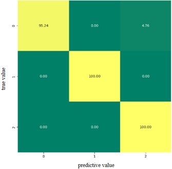
In order to show more intuitively the accurate precision of the proposed model for each classification, the confusion matrix of the fault classification results is plotted. This is shown in Fig. 11, where the horizontal axis represents the diagnostic state and the vertical axis represents the actual fault state.
In the figure, 0-2 corresponds to the 3 state categories, the value on the diagonal line is the recognition accuracy of each state, and the rest of the values are the error rate of recognition. The results in the figure show that the classification accuracy of both category 1 and category 2 is 100 %, and 4.76 % of category 0 is recognized as category 2. It is verified that the method proposed in this paper demonstrates extremely high classification accuracy and stability in the field of rolling bearing fault recognition, and effectively reduces the confusion between categories.
Fig. 11Confusion matrix
4.2. Ablation experiment
In order to further verify the superiority of ADLM in diagnostic classification of rolling bearing faults under complex working conditions, ablation experiments are conducted, which mainly include the following four types:
1) This article presents the ADLM model.
2) Only parallel ACNN, no CFOA BiLSTM.
3) Only CFOA BiLSTM, no parallel ACNN.
4) Replace parallel ACNN with single scale ACNN.
5) Replace BiLSTM with LSTM.
During model training, the learning rate, mini-batch, and training batch were set consistently for each model. The optimizer was the Adam optimizer with a learning rate of 0.0001, the number of training rounds was 50, and the mini-batch size was set to 32. In order to reduce the effect of randomness, each trial was conducted three times. The evaluation criteria are still diagnostic accuracy, F1 score, precision, and recall. The results are shown in Fig. 12 and Table 2.
Fig. 12Comparison of the accuracy of the models
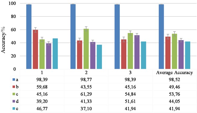
The experimental results strongly confirm the significant advantages and effectiveness of the integrated model proposed in this paper for rolling bearing fault diagnosis. The comparative analysis results show that each module of the model plays an important role in the overall performance. Specifically, when the CFOA-BiLSTM module is removed, the diagnostic accuracy of the model suffers a significant drop of 49.06 %, while the stability is also significantly weakened; similarly, if the parallel ACNN module is removed, the accuracy plummets by 44.76 %, highlighting its importance at the feature extraction level. Simplifying the parallel ACNN to a single ACNN architecture resulted in a 54.47 % decrease in accuracy. And replacing BiLSTM with traditional LSTM plummets the accuracy by 56.68 %, highlighting the important want of BiLSTM in capturing the complex dependencies of time series.
In summary, the ADLM deep learning model proposed in this paper not only demonstrates the powerful ability of ACNN in feature extraction, but also highlights the excellent advantages of CFOA-BiLSTM in processing time series data. The combination of the two significantly improves the effectiveness and stability of rolling bearing fault diagnosis.
Table 2Results of the rubric for each model
Model | Average F1 score / % | Average precision / % | Average recall / % |
a | 98.51±0.18 | 98.56±0.15 | 98.52±0.18 |
b | 40.82±8.74 | 56.71±8.21 | 49.46±7.25 |
c | 52.66±6.15 | 55.23±8.64 | 53.76±6.63 |
d | 32.74±5.84 | 50.41±20.94 | 43.55±6.03 |
e | 34.44±5.53 | 34.36±0.93 | 41.94±3.95 |
5. Discussion
The ADLM model proposed in this paper performs well in rolling bearing fault diagnosis with high accuracy and robustness. Compared with existing studies, the main innovations and advantages of this paper are as follows:
1) Combination of feature extraction and time series analysis: the ADLM module proposed in this paper combines the feature extraction capability of ACNN and the time series analysis capability of CFOA-BiLSTM, which achieves a seamless transition from feature extraction to time series modeling, and is able to capture fault features more comprehensively.
2) Application of optimization algorithm: In this paper, CFOA algorithm is introduced to optimize the hyperparameters of BiLSTM, which significantly improves the performance of the model.
3) Robustness and adaptability: through experimental verification, the model in this paper performs well in rolling bearing fault diagnosis under the background of complex working conditions, and has high robustness and adaptability.
Although this paper has achieved certain research results, there are still some places that can be further improved. Future directions of work include:
1) Further optimize the model structure: explore more efficient feature extraction and time series analysis methods to further improve the performance of the model.
2) Expanding application scenarios: applying the model in this paper to other types of mechanical fault diagnosis, and verifying its applicability and effectiveness in different application scenarios.
3) Improve the optimization algorithm: study more advanced optimization algorithms to further improve the optimization efficiency and accuracy of the model.
6. Conclusions
In this paper, a rolling bearing fault diagnosis model based on ADLM is proposed. The model combines the powerful feature extraction capability of ACNN and the advantages of CFOA-BiLSTM in time series analysis to realize the intelligent diagnosis of rolling bearing faults. Through a large number of experimental verification, the model in this paper performs well in rolling bearing fault diagnosis under the background of complex working conditions, with high accuracy and robustness. The main work and conclusions of this paper are as follows:
1) Method innovation: the ADLM module is designed to capture the spatial features of the bearing vibration signals through the multiscale convolution of ACNN, and combine with the CFOA-optimized BiLSTM for dynamic modeling of timing dependencies, which effectively solves the problem of the traditional method that is difficult to take into account the multiscale features and the time series information.
2) Performance validation: By comparing with mainstream models such as ANN, TCN, MSCNN, etc., the model in this paper improves 61.96 %, 65.19 % and 58.30 % in accuracy, which is significantly higher than the other comparison models.
3) Module contribution: ablation experiments show that the ACNN module can improve the feature characterization ability by 44.76 %, and the CFOA-BiLSTM module improves the timing prediction accuracy by 49.06 %, and the synergistic effect of the two is significantly better than that of a single module or traditional fusion methods.
References
-
Y. Hou, S. Li, and S. Gong, “Filter and improved grey wolf optimization hybrid algorithm for feature selection of rolling bearing faults,” (in Chinese), Computer Integrated Manufacturing System, Vol. 29, No. 5, pp. 1452–1461, 2023.
-
R. Wang, H. Jiang, K. Zhu, Y. Wang, and C. Liu, “A deep feature enhanced reinforcement learning method for rolling bearing fault diagnosis,” Advanced Engineering Informatics, Vol. 54, p. 101750, Oct. 2022, https://doi.org/10.1016/j.aei.2022.101750
-
Z. Fang, Q.-E. Wu, W. Wang, and S. Wu, “Research on improved fault detection method of rolling bearing based on signal feature fusion technology,” Applied Sciences, Vol. 13, No. 24, p. 12987, Dec. 2023, https://doi.org/10.3390/app132412987
-
Y. Qin, R. Yang, H. Shi, B. He, and Y. Mao, “Adaptive fast Chirplet transform and its application into rolling bearing fault diagnosis under time-varying speed condition,” IEEE Transactions on Instrumentation and Measurement, Vol. 72, pp. 1–12, Jan. 2023, https://doi.org/10.1109/tim.2023.3282660
-
Z. Shao et al., “Effect of primary carbides on rolling contact fatigue behaviors of M50 bearing steel,” International Journal of Fatigue, Vol. 179, p. 108054, Feb. 2024, https://doi.org/10.1016/j.ijfatigue.2023.108054
-
L. Wang, Y. Bao, and D. Li, “Wide convolutional deep neural network wind turbine fault diagnosis method based on resampling denoising and principal component analysis,” (in Chinese), Power Generation Technology, No. 6, pp. 824–832, 2023.
-
X. Zhao, L. Zhang, and L. Zhao, “Rolling bearing fault diagnosis using recursive graph coding technique and residual network,” (in Chinese), Journal of Xi’an Jiaotong University, Vol. 57, No. 2, pp. 110–120, 2023.
-
Z. Wang et al., “A high-accuracy fault detection method using swarm intelligence optimization entropy,” IEEE Transactions on Instrumentation and Measurement, Vol. 74, pp. 1–13, Jan. 2025, https://doi.org/10.1109/tim.2024.3502760
-
G.-D. Sun, Y.-R. Wang, C.-F. Sun, and Q. Jin, “Intelligent detection of a planetary gearbox composite fault based on adaptive separation and deep learning,” Sensors, Vol. 19, No. 23, p. 5222, Nov. 2019, https://doi.org/10.3390/s19235222
-
Z. Wang et al., “Few-shot fault diagnosis for machinery using multi-scale perception multi-level feature fusion image quadrant entropy,” Advanced Engineering Informatics, Vol. 63, p. 102972, Jan. 2025, https://doi.org/10.1016/j.aei.2024.102972
-
B. Hu, J. Tang, and J. Wu, “Research on fault diagnosis method of rolling bearings based on triple GAN,” (in Chinese), Noise and Vibration Control, 2021.
-
Z. Wang et al., “A generalized fault diagnosis framework for rotating machinery based on phase entropy,” Reliability Engineering and System Safety, Vol. 256, p. 110745, Apr. 2025, https://doi.org/10.1016/j.ress.2024.110745
-
L. Dong, A. Deng, and Y. Fan, “Fault diagnosis of rolling bearings based on VMD and improved DenseNet,” (in Chinese), Journal of Power Engineering, No. 11, pp. 1500–1505, 2023.
-
Z. Yang, Y. Sun, S. Liu, and J. Jia, “3DSSD: point-based 3D single stage object detector,” in IEEE/CVF Conference on Computer Vision and Pattern Recognition (CVPR), pp. 11030–11039, Jun. 2020, https://doi.org/10.1109/cvpr42600.2020.01105
-
X. Zeng, Q. Gan, and J. Gan, “Fault diagnosis method for rolling bearings based on two-stage fuzzy cognitive map,” (in Chinese), Electromechanical Engineering, Vol. 40, No. 5, pp. 731–738, 2023.
-
H. Jia, Q. Wen, Y. Wang, and S. Mirjalili, “Catch fish optimization algorithm: a new human behavior algorithm for solving clustering problems,” Cluster Computing, Vol. 27, No. 9, pp. 13295–13332, Jun. 2024, https://doi.org/10.1007/s10586-024-04618-w
About this article
This study was supported by the Henan Provincial Science and Technology Research Project (252102240042) and the National Natural Science Foundation for Young Scientists (62403254).
The datasets generated during and/or analyzed during the current study are available from the corresponding author on reasonable request.
Ruijun Zhang: methodology, software, writing-review and editing. Rui Li: writing-original draft, conceptualization. Chuan Liu: validation, formal analysis, investigation. Jing Zhu: validation, formal analysis, investigation, funding acquisition. Yaowei Shi: validation, formal analysis, investigation, funding acquisition.
The authors declare that they have no conflict of interest.
