Abstract
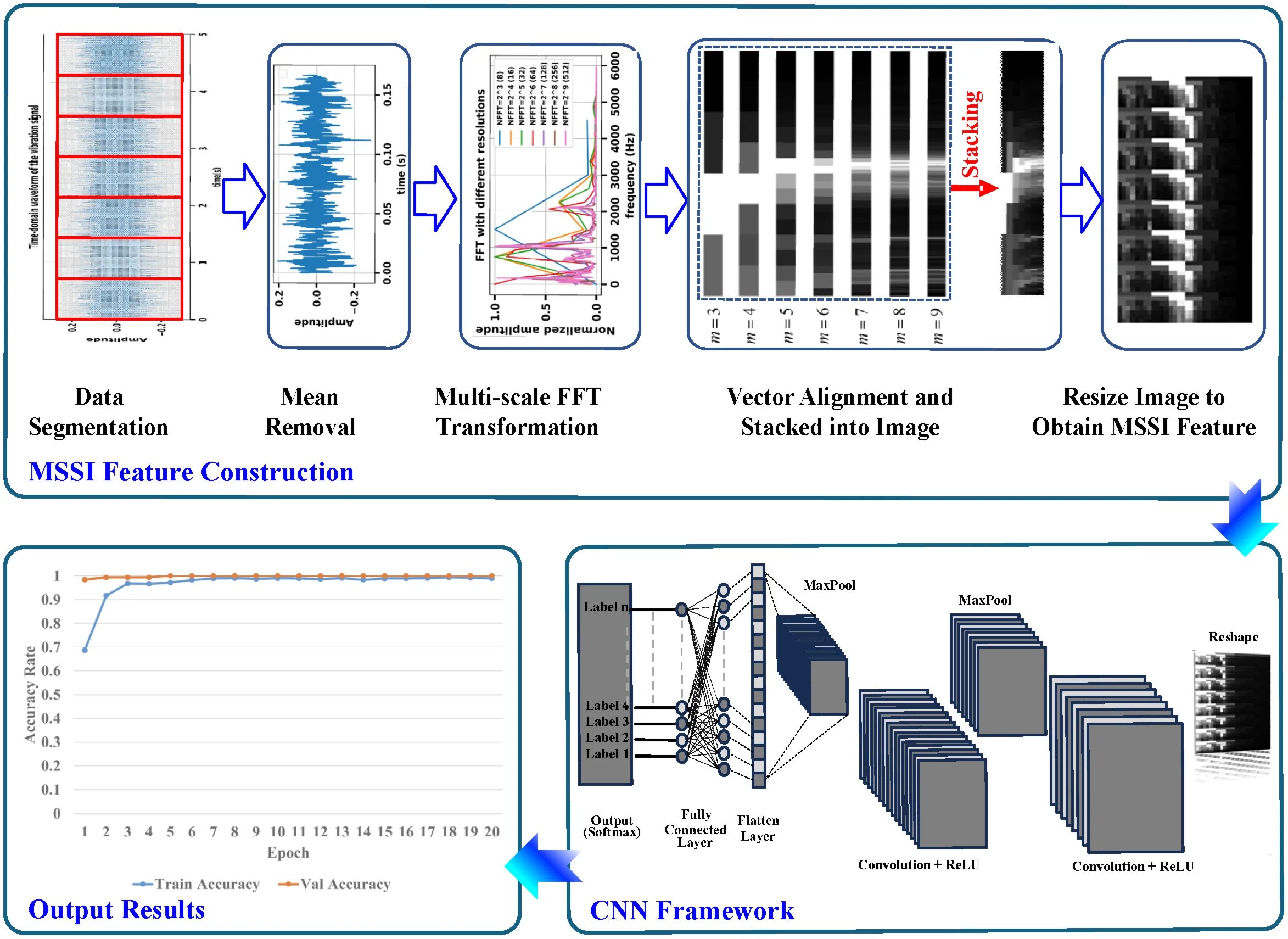
To address the challenges of poor performance in traditional diagnosis methods and two-dimensional (2-D) feature based approaches, this paper proposes a novel fault diagnosis approach based on multi-scale spectrum feature images and deep learning. Firstly, the vibration signal is preprocessed through mean removal processing and then converted to multi-length spectrum with fast Fourier transform (FFT). Secondly, a novel 2-D feature called multi-scale spectral image (MSSI) is constructed by multi-length spectrum paving scheme. Finally, a deep learning framework, convolutional neural network (CNN), is formulated to diagnose the bearing faults. Two experimental cases are utilized to verify the effectiveness of the proposed method. Experimental results demonstrate that the proposed method significantly improves the accuracy of fault diagnosis.
Highlights
- A novel two-dimensional (2-D) feature, termed the multi-scale spectral image (MSSI), is proposed to extract comprehensive frequency-domain representations of bearing vibration signals by directly deriving multiscale spectral information with different resolution levels.
- A bearing fault diagnosis framework is developed by integrating the MSSI feature with a lightweight convolutional neural network (CNN) architecture.
- The proposed MSSI feature demonstrates superior performance over conventional features, even surpassing that of time-frequency images integrated with advanced deep learning models, such as ResNet-18.
1. Introduction
Rotating machinery is widely utilized in various fields such as construction, aviation, power generation, and metallurgy. Mechanical failures can result in significant economic losses and pose risks to the workers’ safety [1]. As a critical component of rotating machinery, the reliability of rolling bearings plays a decisive role in the operational state of the machinery, particularly concerning fatigue life, friction torque, and vibration performance [2-4]. Hence it is of great importance to diagnose bearing faults immediately.
Vibration analysis is one of the most commonly used methods in the fault diagnosis of rotating machinery because the vibration signal can reflect the dynamic characteristics of the system and be both sensitive to faults and easy to measure [5]. Feature extraction and fault classification are two critical procedures in bearing fault diagnosis. Many researches have been devoted to exploring how to extract more effective features and construct more efficient identification methods for fault diagnosis in the past few decades. In existing methods, fault features are primarily constructed using time-domain, frequency-domain, and time-frequency domain feature extraction techniques, such as kurtosis analysis, cepstrum analysis, wavelet analysis, and so on [6-8]. These features typically take the form of scalars or vectors, which leads to a limited capability for health information mining. Therefore, two-dimensional (2-D) features are tentatively constructed in different ways to extract more fault information. For example, Li et al. [9] proposed to diagnose bearing faults using spectrum images of vibration signals. Guo et al. [10] extracted continuous wavelet transform scalogram as 2-D feature to conduct fault diagnosis for rotating machinery. Nie et al. [11] proposed to transform the vibration signals of multi-channel sensors into RGB images as fault features for bearing fault diagnosis. The 2-D feature based methods seem to be more robust and effective for machine fault diagnosis even in the case of limited data scarcity. Once the fault features are extracted, pattern recognition models can be employed to achieve fault diagnosis, such as statistical models, machine learning models, and so on [12], [13]. In recent years, the rapid development of deep learning technologies has significantly enhanced the potential of 2-D feature based methodologies in machine fault diagnosis. A novel research trend has emerged, which involves the conversion of vibration signals into images and the application of deep learning models for the automatic extraction of image features to facilitate fault diagnosis. This innovative approach not only effectively addresses the constraints inherent in conventional methods but also attains a superior level of diagnostic precision. However, existing 2-D feature construction techniques often rely on single-scale representations, which may not adequately capture the frequency diversity of bearing vibration signals. Moreover, handcrafted 2-D transformations such as continuous wavelet transform or spectrograms may still depend heavily on parameter settings and expert knowledge, which limit the generalizability and scalability of such methods.
To address these limitations, we propose a novel fault diagnosis method using multi-scale spectral images and deep learning technology in this paper. In the proposed method, considered that the spectral components and frequency structures of bearings typically vary with different component fault conditions, a new 2-D feature called multi-scale spectral image (MSSI) is constructed by multi-length spectrum paving strategy to depict different health states of bearings. Then a deep learning approach, convolutional neural network (CNN), is employed to model and identify faults using the extracted MSSI features.
The main contributions of this work are summarized as follows: (1) a novel 2-D feature, namely MSSI, is proposed to extract comprehensive frequency-domain representations of bearing signals, which is derived directly from the spectrum with different frequency resolution levels and enhances the descriptive capability of the features by preserving both global and local spectral characteristics, thereby providing a more informative depiction of the bearing health states; (2) a fault diagnosis methodology using the MSSI feature combined with a lightweight CNN architecture is proposed to diagnose bearing faults.
The remainder of this paper is organized as follows. The process of MSSI feature extraction is explained in detail in section 2. Section 3 provides the overall procedure for bearing fault diagnosis with MSSI and CNN. Section 4 gives the experimental verification results using two bearing datasets. Finally, the conclusion of this work is given in section 5.
2. MSSI feature extraction
2.1. Overview of FFT algorithm
The Fourier transform is one of the fundamental methods for transforming time-domain series to frequency-domain. The frequency spectrum information of the signal at discrete frequency points can be obtained through discrete Fourier transform (DFT) processing. For a discrete-time signal , its DFT is defined as follows:
where .
Fast Fourier transform (FFT) is an efficient algorithm for computing the DFT. When the number of data points is (where is a positive integer), it can reduce computing complexity dramatically for analyzing data using FFT. To lay the foundation for constructing MSSI features in subsequent stages, FFT is applied for generating spectrum with different frequency resolutions, which is achieved by taking different values of in in this study.
2.2. Construction of the MSSI feature
The frequency spectrum contains a large amount of characteristic information about the running process of a bearing, such as the fault characteristic frequencies and their harmonics, the geometrical structure of the spectrum, and so on. Aiming at mining the health information contained in the spectrum as much as possible, a novel feature named MSSI is innovatively constructed by generating a series of spectrum using different frequency resolutions. The construction process of the proposed MSSI feature is presented in Fig. 1.
First, the collected original vibration data are first divided into sub-signals and then the signals are detrended through mean removal processing.
Second, multi-scale FFT transformation is performed to obtain the spectrum with FFT using different frequency resolutions, which achieved by setting the variable in section 2.1 as different positive integers. And the variable is set 3 to 9 in this paper. In addition, all spectrum sequences are pre-processed using the maximum-minimum normalization method to eliminate the effects of different magnitudes for MSSI construction.
Fig. 1Construction process of the proposed MSSI feature
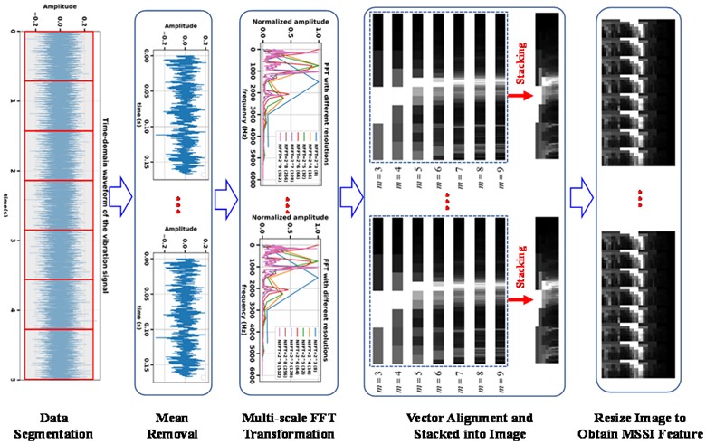
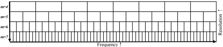
Third, since the length of spectrum sequences vary with frequency resolutions, the vector alignment processing is performed on the aforementioned sequence. All spectrum sequences will be of the same length to facilitate subsequent construction of MSSI feature. In this study, the elements in shorter vectors are uniformly replicated to extend their lengths to match the reference sequence namely the longest one, through proportional element duplication. Then these aligned sequences are stacked into an image in order. An example of the vector alignment processing and vector stacking is presented in Fig. 2. Suppose that there are four series generated with 4-7, the first three sequences are aligned to the last one that served as the reference during the alignment process. Subsequently, these aligned sequences are ordered into a matrix to obtain the image feature.
Finally, the above-mentioned image feature is usually an elongated image, which is not conducive to the further processing for the image features and the final fault diagnosis. Therefore, the image features obtained in the previous step are resized to an approximately square image (with size 56×32 in pixels in this study), which is called as the MSSI feature.
3. Fault diagnosis with MSSI and CNN
The MSSI feature, as a new 2-D feature, comprehensively depict the health information from the frequency spectrum of bearing vibration signals. Deep learning technology is employed to process these image features, and a lightweight CNN model is applied for image classification to diagnose bearing faults in our research.
Fig. 2An example of vector alignment and vectors stacking into an image
3.1. CNN model design
This network framework is inspired by the typical LeNet-5 [14] and the proposed CNN architecture is based on the same strategy, using convolutional and pooling layers to extract image features and fully connected layers for classification.
Fig. 3The proposed CNN framework
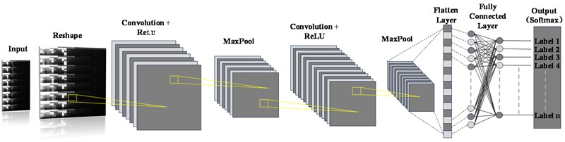
Compared to the original LeNet-5, this network makes a series of changes in detail, including different number of convolutional kernels and layers, and introduces a dropout layer to mitigate the risk of overfitting [15]. To facilitate feature extraction and classification using CNN model, an input image of size 56×32 (in pixels) is first reshaped to a 128×128 (in pixels) image by nearest neighbor interpolation. The proposed CNN framework is presented in Fig. 3.
Table 1Parameters of the proposed CNN architecture
No. | Layer type | Number of filters | Filters size | Stride | Zero Padding | Outputs |
1 | Input | – | – | – | – | (128, 128, 1) |
2 | Conv1 | 16 | 3×3 | 1 | Yes | (128, 128, 16) |
3 | Max Pool | – | 2×2 | 2 | – | (64, 64, 16) |
4 | Conv2 | 32 | 3×3 | 1 | Yes | (64, 64, 32) |
5 | Max Pool | / | 2×2 | 2 | – | (32, 32, 32) |
6 | FC1 | – | – | – | – | (256, 1) |
7 | FC2 | – | – | – | – | (10, 1) |
The parameters of the proposed CNN architecture are shown in Table 1. In this research, we design two convolutional layers. The kernel size for both layers is 3×3, and the stride is set to 1 by default. The first convolutional layer (Conv1) uses 16 kernels, while the second convolutional layer (Conv2) contains 32 kernels, which enhances the model's feature learning capacity. Zero padding is applied to ensure that the input and output sizes remain unchanged, which adds zeros around the borders of the input volume. It is used to maintain the same spatial dimensions between the input and output volumes, thereby preserving as much information as possible from the original input [14]. The calculation formula of the convolutional layer is as follows:
where represents the value of the input feature at position , represents the weight of the convolution kernel at and represents the bias, represents the value of the output feature map at position . is the size of the convolution kernel and represents the stride. In convolutional layer, is set to 1 by default and is set to 3×3. represents the padding and the calculation formula of the output feature map as follows:
where and represents the height and width of the input feature map, which is 128×128, and represents the height and width of the output feature map, which is 128×128, according to the formula we can get equals 1.
Additionally, two Max Pooling layers are incorporated, with a kernel size of 2×2 and a stride of 2. This pooling operation preserves the most significant features in the input feature map, while reducing its size, thereby decreasing the computational burden of subsequent layers. The expression of the maximum pooling layer in the pooling layer is as follows:
where represents the stride in the pooling layer, which is set to 2, and are the length and width of the pooling kernel, which is 2×2.
After the input image passes through the convolution layer and the pooling layer, it needs to rely on the fully connected layer to classify the extracted features. In the fully connected layer, all input feature maps are expanded into one-dimensional feature vectors, weighted summed and activated by the activation function. We add two fully connected layers, FC1 and FC2, are designed, with FC1 consisting of 256 neurons and FC2 containing 10 neurons. Since FC2 serves as both the fully connected layer and the output layer, it is designed with 10 neurons to match the number of output classes. The fully connected layer can be expressed as follows [16]:
where represents the output of the neuron and represents the activation function and represents the th fully connected layer and represents the weight matrix connecting the th layer to the layer and represents the output vector from the th layer and represents the bias.
The cross-entropy loss function is applied in our research, which includes the softmax function, so the softmax is not explicitly applied in the model, and an L2 regularization parameter of 0.0001 is applied, to enhance the model performance and generalization. The cross-entropy loss function can be represented as follows [17]:
where represents the number of classes and represents truth label and represents the probability predicted by the model and represents the weight parameter matrix of the neural network and represents the L2 norm of the weight and represents the weight decay, which is set to 0.0001.
A dropout layer with a dropout rate of 0.5 is introduced to prevent overfitting. The Adam optimizer is employed with a learning rate of 0.001. The hyperparameter information of the proposed CNN structure is summarized in Table 2.
Table 2Hyperparameters of the proposed CNN
Hyperparameters | Value |
Dropout | 0.5 |
Activation Function | ReLU |
Loss Function | Cross-Entropy Loss |
Optimizer | Adam |
Learning Rate | 0.001 |
Weight Decay | 0.0001 |
Epoch | 20 |
Batch Size | 10 |
3.2. The proposed fault diagnosis scheme
The diagnosis model is first established using the MSSI features derived from the offline vibration data and deep learning technology in the offline training procedure. Then the bearing health states can be diagnosed with the trained model by inputting the MSSI features derived from the online monitoring data. The main process can be summarized as follows.
(1) MSSI Feature Extraction: The MSSI features of the offline or the online vibration signals are constructed using the method in Section 2.
(2) CNN Model Building: The CNN parameters are initialized at first, and the MSSI features of the offline data are input to the CNN. Then the forward propagation algorithm is used to calculate the training error and the back propagation algorithm to obtain the error and gradients. Finally, the parameters are adjusted according to the obtained error and gradients to optimize the CNN model, thereafter a trained CNN model is obtained and can be applied for final fault diagnosis.
(3) Online Fault Diagnosis: The MSSI feature of an online data sample is input to trained CNN model to diagnose the corresponding health state of bearing.
The overall flowchart of the proposed fault diagnosis scheme is shown in Fig. 4.
4. Experimental results
To validate the reliability and generalization capability of the proposed method, two distinct datasets were employed in the experiments: the widely used CWRU dataset, in which bearings are fixed via the outer ring, and a conveyor idler dataset, acquired under an inner ring fixing condition. These datasets covers two different bearing installation configurations.
4.1. Case analysis on CWRU data
4.1.1. Introduction to CWRU bearing data
This validation data comes from the publicly available rolling bearing dataset from Case Western Reserve University (CWRU) [18]. As shown in Fig. 5, the test rig consists of a 2 hp motor (left), a torque transducer/encoder (center), a dynamometer (right), and control electronics (not shown). The testing bearing were installed on the motor housing at the drive end of the motor and the bearing outer ring was attached with the motor housing. The vibration signals were acquired using acceleration transducer. Four bearing health state (normal, inner race fault, rolling element fault, and outer race fault) and four levels of fault severity (7 mils, 14 mils, 21 mils and 28 mils) are considered in the experiment. And the vibration data under four different load/speed conditions (Load0 = 0 hp/1797 rpm, Load1 = 1 hp/1772 rpm, Load2 = 2 hp/1750 rpm and Load3 = 3 hp/1730 rpm) were sampled using the accelerometers attached to the drive end of the motor housing with 12 kHz sampling rate.
Fig. 4Flow chart of fault diagnosis based on MSSI and CNN

Fig. 5The test rig for CWRU bearing data [18]
![The test rig for CWRU bearing data [18]](https://static-01.extrica.com/articles/24934/24934-img5.jpg)
In order to facilitate the MSSI for extracting more fault information and enrich the data set, a data division strategy is employed for data segmentation shown in Fig. 1, in which a length of about 1/6 second data is applied for data segmentation. In other words, it can be guaranteed that a single sample could contain vibration data of five shaft rotations. This temporal span guarantees the comprehensive acquisition of bearing signals.
4.1.2. Results analysis
A comprehensive ten class diagnosis problem is employed to evaluate the performance of the proposed method. This instance involves fault type diagnosis and fault severity diagnosis, which makes it the most challenging diagnostic problem using the CWRU data. Here several diagnosis cases under single running condition and multiple running conditions are employed for validation analysis. As shown in Table 3, vibration datasets under four running conditions (Load0, Load1, Load2 and Load3) are represented by A, B, C and D, respectively. And the vibration datasets under Load0-Load3 conditions is designated as E. The sample number under different running conditions is different due to the different lengths of the original data. The sample number of the normal state under Load0 is 120, while the sample number of the normal state under Load1, Load2 or Load3 is 240. The sample number of other health states is 60 or 61. Meanwhile, 70 % of the total samples is randomly selected as the training set for constructing CNN model and the remaining 30 % as the testing set for examining model classification ability.
Table 3Description of the CWRU bearing datasets
Health state | Normal | Inner race fault | Ball fault | Outer race fault | ||||||||
Fault diameter (mil) | 0 | 7 | 14 | 21 | 7 | 14 | 21 | 7 | 14 | 21 | ||
Classification label | NM | IR1 | IR2 | IR3 | B1 | B2 | B3 | OR1 | OR2 | OR3 | ||
Dataset A | Load0 | Train | 84 | 42 | 42 | 43 | 43 | 42 | 42 | 42 | 42 | 43 |
Test | 36 | 18 | 18 | 18 | 18 | 18 | 18 | 18 | 18 | 18 | ||
Dataset B | Load1 | Train | 168 | 42 | 42 | 42 | 42 | 43 | 42 | 43 | 43 | 42 |
Test | 72 | 18 | 18 | 18 | 18 | 18 | 18 | 18 | 18 | 18 | ||
Dataset C | Load2 | Train | 168 | 43 | 42 | 42 | 42 | 42 | 43 | 42 | 42 | 43 |
Test | 72 | 18 | 18 | 18 | 18 | 18 | 18 | 18 | 18 | 18 | ||
Dataset D | Load3 | Train | 168 | 43 | 42 | 42 | 42 | 43 | 43 | 43 | 42 | 42 |
Test | 72 | 18 | 18 | 18 | 18 | 18 | 18 | 18 | 18 | 18 | ||
Dataset E | Load0-Load3 | Train | 588 | 170 | 168 | 169 | 169 | 170 | 170 | 170 | 169 | 170 |
Test | 252 | 72 | 72 | 72 | 72 | 72 | 72 | 72 | 72 | 72 | ||
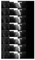
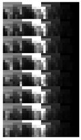
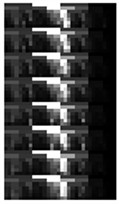
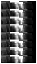
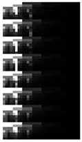
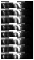
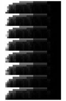
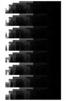
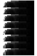
The MSSI features were first extracted from both the training set and the testing set using the method presented in section 2. In order to present the proposed MSSI features intuitively, an example of MSSI feature for the ten health states under Load0 condition is given in Fig. 6. The MSSI features of ten health conditions are visualized after reshaping the original 7×256 spectral representations into 56×32 grayscale images. As presented in Fig. 6, the row axis corresponds to frequency components ranging from low to high, while the column axis denote spectral energy distribution under different frequency resolution in a specific frequency band, where each group of rows (8-pixel height) reflects the spectral response under a specific FFT length (from 23 to 29).
To quantitatively characterize these differences, mean gray value (representing the average pixel intensity of the image), standard deviation (quantifying the dispersion of pixel intensities and thus reflecting image contrast and detail), and information entropy (measuring the randomness or information content of the pixel intensity distribution), were employed for further quantitative analysis. In particular, the information entropy is a classic statistic that measures the uncertainty of grayscale distribution in an image and is widely used to describe the complexity and information richness of an image. For the normalized images in the range in this study, it is necessary to discretize the normalized values into a finite set of gray levels prior to entropy computation. This is typically achieved by mapping each normalized pixel value to an integer grayscale level by . Then the information entropy can be calculated as follows:
where represents the information entropy of the image and represents the appearing probability of gray level 𝑘, which is calculated as the number of pixels with gray value 𝑘 divided by the total number of pixels in the image.
Table 4 summarizes three statistical metric values under different health conditions shown in Fig. 6. These metrics provide objective evidence supporting the qualitative observations and further distinguish the fault types based on their spectral image characteristics. Also, it can be seen that there are relatively obvious differences between the MSSI features for different health states.
Fig. 6An example of MSSI feature for the ten health states under Load0 condition
a) B1
b) B2
c) B3
d) IR1
e) IR2
f) NM
g) OR1
h) OR2
i) OR3
j) IR3
Table 4Three statistical metrics under different health conditions
Metrics | NM | B1 | B2 | B3 | IR1 | IR2 | IR3 | OR1 | OR2 | OR3 |
Mean gray value | 0.151 | 0.206 | 0.247 | 0.222 | 0.313 | 0.307 | 0.199 | 0.192 | 0.249 | 0.268 |
Standard deviation | 0.272 | 0.275 | 0.287 | 0.27 | 0.309 | 0.313 | 0.288 | 0.294 | 0.27 | 0.305 |
Information entropy | 4.76 | 5.73 | 5.91 | 5.86 | 6.18 | 6.22 | 5.62 | 5.39 | 6.80 | 6.01 |
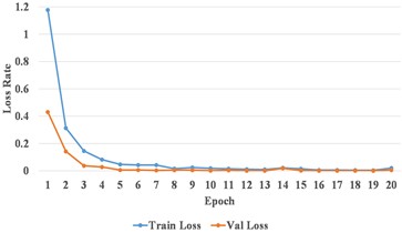
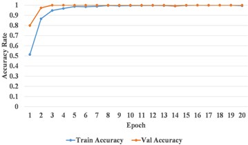
After all MSSI features were extracted, the randomly selected training samples under different load/speed conditions were applied to train the CNN model. An example of the training process of CNN model for Dataset E is given in Fig. 7. It can be seen that the loss rate drops rapidly and remains in a very small range, and both the train and validation accuracies are approximate to 100.00 % after about the 7th epoch.
Fig. 7An example of the training process of CNN model for Dataset E
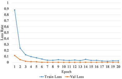
a) Loss curve
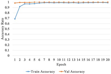
b) Accuracy curve
Then the remaining testing samples were input to the trained CNN model to validate the effectiveness of the proposed fault diagnosis scheme. Ten trials were conducted to record the classification results and compute the average diagnostic accuracy. The accuracy results of the CWRU bearing set are presented in Table 5 and Table 6. In the context of diagnostic case analysis under single running conditions, the testing samples from Dataset A, B, C and D were classified with average accuracy of 99.80 %, 99.87 %, 100.00 % and 99.96 %, respectively. For the diagnostic cases under multiple running conditions, the proposed framework exhibits robust performance with 99.99 % classification accuracy for Dataset E. Examining the results, it can be observed that most testing samples are classified correctly and the proposed method demonstrates consistently high accuracy across all running conditions.
Table 5Experimental results for single running condition
Dataset | Average accuracy | Standard deviation |
A | 99.80 % | 0.350 % |
B | 99.87 % | 0.400 % |
C | 100.00 % | 0.000 % |
D | 99.96 % | 0.140 % |
Table 6Experimental results for multiple running conditions
Dataset | Testing accuracy | Total accuracy | Standard deviation | |||
Load0 | Load1 | Load2 | Load3 | |||
E | 99.95 % | 100.00 % | 100.00 % | 100.00 % | 99.99 % | 0.026 % |
As shown in Table 5 and Table 6, it can also be shown that the results demonstrate inferior performance on Dataset A and Dataset B. The confusion matrices of the CNN models for Dataset A and Dataset B are presented in Fig. 8. It can be observed that the models are generally effective in distinguishing between different fault types. However, there exists a potential misclassification of B2 as B1 in Dataset A; similarly, B3 in Dataset B may have been erroneously classified as B1. The main reason could be that the impact energy generated by the defects of the rolling elements is weak and significantly lower than that of the other faults (e.g. the inner race or outer race faults) especially under light-load conditions, which results in a relatively poor discrimination in the spectrums and the MSSI features.
Fig. 8The confusion matrices of CNN model for Dataset A and Dataset B
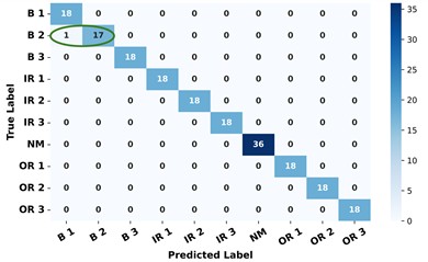
a) Confusion matrix for Dataset A
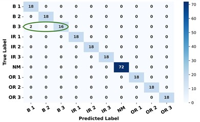
b) Confusion matrix for Dataset B
4.2. Case analysis on a conveyor idler dataset
4.2.1. Introduction to the conveyor idler testbed
The test bench shown in Fig. 9 consists of an AC motor, a frequency converter, a conveyor idler, a tachometer, an accelerometer, a signal acquisition instrument and a computer [19]. A normal bearing (6204 type) is installed on one end and the test bearing is installed on the other end (the right end shown in Fig. 9) of the conveyor idler, which is driven by a belt through the AC motor. The bearing inner ring was attached with the idler shaft. The type of both normal and tested bearings is 6204. Five bearing health states (normal, inner race fault, rolling element fault, outer race fault and cage fault) are considered in the experiment, and the vibration signals at a motor speed of 1080 rpm were collected using the sensors and the signal acquisition instrument with 20 kHz sampling frequency. One million data points (i.e., 50 s) were recorded in a sampling signal and the signals were sampled twice for different bearing health states of the conveyor idler. More details about the experimental platform can refer to [19].
Fig. 9Test bench of the belt conveyor idler [19]
![Test bench of the belt conveyor idler [19]](https://static-01.extrica.com/articles/24934/24934-img20.jpg)
4.2.2. Results analysis
Similarly, to enhance the capability of MSSI in extracting fault-related information, a data division strategy is implemented for segmentation, as illustrated in Fig. 1. Each sample is ensured to contain vibration data corresponding to about seven shaft rotations, where this duration is sufficient to ensure the comprehensive acquisition of conveyor idler signals. Therefore, a total of 298 samples are obtained for each of the five health states. Similarly, 70 % of the total samples is randomly selected to train the CNN model and the remaining 30 % is applied for testing the model diagnostic ability. The sizes of datasets for different health states are presented in Table 7.
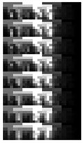
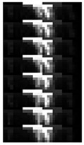
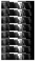
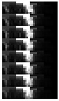
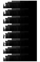
An example of MSSI features for the conveyor idler bearing under different health states is presented in Fig. 10. It is evident that the characteristic differences can still be depicted between the MSSI features for different fault types. The MSSI features derived from training set were used to train the CNN model. Also, an example of the CNN training process is presented in Fig. 11. It can be observed that the loss rate decreases rapidly and stabilizes within a narrow range, while both the training and validation accuracies approach 100.00 % after approximately the 8th epoch.
Table 7Description of the conveyor idler bearing datasets
Label | Health state | Training set | Testing set |
IR | Inner race fault | 209 | 89 |
B | Rolling element fault | 209 | 89 |
OR | Outer race fault | 209 | 89 |
NM | Normal | 209 | 89 |
CA | Cage fault | 209 | 89 |
Total | / | 1045 | 445 |
Table 8Accuracy results of the conveyor idler bearing analysis
Label | IR | B | OR | NM | CA | Average accuracy | Standard deviation |
Accuracy | 100.00 % | 100.00 % | 100.00 % | 100.00 % | 100.00 % | 100.00 % | 0.000 % |
Once the CNN model is built, the testing samples were input to validate the performance of the proposed method. Then ten trials were conducted to obtain average results, ensuring the outcomes are generalizable and not influenced by special cases. The accuracy results are shown in Table 8. It can be seen that all the testing samples were classified with 100 % accuracy. This further substantiates the reliability and validity of the methodology proposed in this paper.
Fig. 10An example of MSSI features for the conveyor idler bearing under different health states
a) NM
b) IR
c) OR
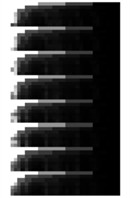
d) B
e) CA
Fig. 11An example of the training process of CNN model for conveyor idler bearing
a) Loss curve
b) Accuracy curve
4.3. Discussion
According to the experimental results, the proposed method demonstrates high diagnostic accuracy on both the CWRU dataset and the conveyor idler dataset. However, for the CWRU dataset, the classification accuracies under Load0 and Load1 conditions are relatively lower. As indicated by the corresponding confusion matrices, there is a tendency for misclassification between B1 and B2 under Load0, and between B1 and B3 under Load1. This is primarily attributed to the high similarity in fault features among rolling element defects of different sizes within the same fault type. Such similarity poses challenges for accurate discrimination using the proposed method to diagnose different fault severities.
In order to further compare the reliability and the potential application of the proposed scheme, a comparative study between current work and some published works is presented in Table 9. These published methods are all verified and the ten classifications problem under single and/or multiple operational scenarios are considered with the same CWRU bearing data. As presented in Table 9, bearing faults were diagnosed with GAF-CA-CNN model using GAF image as feature in [20]. In [17], time-frequency images were extracted and applied for fault diagnosis, and bearing faults were diagnosed with CNN, ResNet-18 or RNELM models. In [21], ensemble deep neural network and CNN is proposed as model for bearing fault diagnosis using vibration signal and statistical feature. A detailed result comparison between this work and those published works is presented in Table 9. It can be seen that the proposed scheme shows better performance for bearing fault diagnosis than the others. Furthermore, only using a lightweight CNN, the proposed MSSI feature is evidently superior to other features, even to the time-frequency image combined with some advanced models, such as ResNet-18 or RNELM presented in [17]. This indicates that the proposed MSSI feature is a more promising and effective 2-D feature for bearing fault diagnosis.
Otherwise, the time costs of MSSI feature construction, model training, and model diagnosis were calculated to evaluate the feasibility of industrial implementation of the proposed method. All tests were conducted using MATLAB R2024b and PyCharm Community Edition 2023.1.3. Specifically, MATLAB was employed for preprocessing the time-series vibration signals and generating MSSI features. Subsequently, the extracted feature were utilized for model training and fault diagnosis with PyCharm, leveraging the PyTorch framework (version 2.4.1 + cu124). The detailed hardware and software configurations are summarized in Table 10.
Table 9Comparison between our method and some published methods
Reference | Method | Training | Testing | Condition | Accuracy |
[20] | GAF image + GAF-CA-CNN | 9000 | 1000 | Load0 | 99.62 % |
[17] | Time-frequency image + CNN | 4000 | 1000 | Load0-Load3 | 95.00 % |
Time-frequency image + ResNet-18 | 4000 | 1000 | Load0-Load3 | 98.10 % | |
Time-frequency image + RNELM | 4000 | 1000 | Load0-Load3 | 99.90 % | |
[21] | Vibration signal and statistical feature + CNNPEDNN | 2000 | 370 | Load0 | 95.76 % |
2000 | 370 | Load1 | 97.92 % | ||
2000 | 370 | Load2 | 97.62 % | ||
2000 | 370 | Load3 | 98.10 % | ||
Current work | MSSI feature + CNN | 465 | 198 | Load0 | 99.80 % |
549 | 234 | Load1 | 99.87 % | ||
549 | 234 | Load2 | 100.00 % | ||
550 | 234 | Load3 | 99.96 % | ||
2113 | 900 | Load0-Load3 | 99.99 % |
Table 10Hardware and software configuration environment parameters
Hardware / Software | Configure |
Operating system | Windows 11 (64-bit) |
CPU | 12th Gen Intel(R) Core(TM)i7-12700H |
GPU | NVIDIA GeForce RTX 3060 Laptop |
Development platform | MATLAB 2024b |
PyCharm Community Edition 2023.1.3 | |
Development framework | Torch 2.4.1 + cu124 |
Here, the time cost evaluations were conducted using CWRU data from Load0 condition as an example to evaluate the time consumption at different stages of the process. The results are presented in Table 11.
According to Table 11, the average time required for the MSSI feature construction is approximately 0.1831 seconds per sample. The model training phase has a total duration of 5.273 seconds for 20 epochs, and the average training time per epoch is approximately 0.2637 seconds. In the diagnosis stage, the model demonstrates high computational efficiency, with an average inference time of only 0.0014 seconds per testing sample. The experimental results demonstrate that both the MSSI construction process and CNN-based diagnosis exhibit significantly low computational time consumption, which substantiates the industrial applicability of the proposed methodology.
Table 11Time cost evaluation results for different phase
Phase | Sample size | Total time | Average time |
MSSI construction | 663 samples | 121.398 s | 0.1831 s/sample |
CNN training | 465 samples / 20 epochs | 5.273 s | 0.2637 s/epoch |
CNN diagnosis | 198 samples | 0.285 s | 0.0014 s/sample |
5. Conclusions
In this paper, a novel feature, multi-scale spectral image (MSSI), is proposed as a 2-D feature to represent different health states for bearing fault diagnosis. The MSSI is constructed with the FFT algorithm using a multi-length spectrum paving strategy, where abundant information contained in multi-scale spectrum are deeply exploited for the representation of bearing health states. Then a new scheme is proposed for bearing fault diagnosis using a lightweight CNN architecture. The proposed method is applied to two datasets: the CWRU bearing dataset and a conveyor idler fault dataset. Compared to other fault diagnosis methods, the proposed approach demonstrates high classification performance, offering a novel solution for bearing fault diagnosis.
References
-
F. Gougam, C. Rahmoune, D. Benazzouz, and B. Merainani, “Bearing fault diagnosis based on feature extraction of empirical wavelet transform (EWT) and fuzzy logic system (FLS) under variable operating conditions,” Journal of Vibroengineering, Vol. 21, No. 6, pp. 1636–1650, Sep. 2019, https://doi.org/10.21595/jve.2019.20092
-
C. Che, H. Wang, X. Ni, and Q. Fu, “Domain adaptive deep belief network for rolling bearing fault diagnosis,” Computers and Industrial Engineering, Vol. 143, p. 106427, May 2020, https://doi.org/10.1016/j.cie.2020.106427
-
F. Meng et al., “Reliability evaluation of rolling bearings based on generative adversarial network sample enhancement and maximum entropy method,” Scientific Reports, Vol. 14, No. 1, p. 31185, Dec. 2024, https://doi.org/10.1038/s41598-024-82452-1
-
J. Xie, G. Du, C. Shen, N. Chen, L. Chen, and Z. Zhu, “An end-to-end model based on improved adaptive deep belief network and its application to bearing fault diagnosis,” IEEE Access, Vol. 6, pp. 63584–63596, Jan. 2018, https://doi.org/10.1109/access.2018.2877447
-
J. Park et al., “An image-based feature extraction method for fault diagnosis of variable-speed rotating machinery,” Mechanical Systems and Signal Processing, Vol. 167, p. 108524, Mar. 2022, https://doi.org/10.1016/j.ymssp.2021.108524
-
J. Prakash Kumar, P. S. Chauhan, and P. Prakash Pandit, “Time domain vibration analysis techniques for condition monitoring of rolling element bearing: A review,” Materials Today: Proceedings, Vol. 62, pp. 6336–6340, Jan. 2022, https://doi.org/10.1016/j.matpr.2022.02.550
-
S. Gawde, S. Patil, S. Kumar, P. Kamat, K. Kotecha, and A. Abraham, “Multi-fault diagnosis of industrial rotating machines using data-driven approach: a review of two decades of research,” Engineering Applications of Artificial Intelligence, Vol. 123, p. 106139, Aug. 2023, https://doi.org/10.1016/j.engappai.2023.106139
-
B. Wang, H. Li, X. Hu, and W. Wang, “Rolling bearing fault diagnosis based on multi-domain features and whale optimized support vector machine,” Journal of Vibration and Control, Vol. 31, No. 5-6, pp. 708–720, Feb. 2024, https://doi.org/10.1177/10775463241231344
-
W. Li, M. Qiu, Z. Zhu, B. Wu, and G. Zhou, “Bearing fault diagnosis based on spectrum images of vibration signals,” Measurement Science and Technology, Vol. 27, No. 3, p. 035005, Mar. 2016, https://doi.org/10.1088/0957-0233/27/3/035005
-
S. Guo, T. Yang, W. Gao, and C. Zhang, “A novel fault diagnosis method for rotating machinery based on a convolutional neural network,” Sensors, Vol. 18, No. 5, p. 1429, May 2018, https://doi.org/10.3390/s18051429
-
G. Nie, Z. Zhang, Z. Jiao, Y. Li, M. Shao, and X. Dai, “A novel intelligent bearing fault diagnosis method based on image enhancement and improved convolutional neural network,” Measurement, Vol. 242, p. 116148, Jan. 2025, https://doi.org/10.1016/j.measurement.2024.116148
-
A. A. Soomro et al., “Insights into modern machine learning approaches for bearing fault classification: A systematic literature review,” Results in Engineering, Vol. 23, p. 102700, Sep. 2024, https://doi.org/10.1016/j.rineng.2024.102700
-
D. Neupane, M. R. Bouadjenek, R. Dazeley, and S. Aryal, “Data-driven machinery fault diagnosis: A comprehensive review,” Neurocomputing, Vol. 627, p. 129588, Apr. 2025, https://doi.org/10.1016/j.neucom.2025.129588
-
Z. Chen, A. Mauricio, W. Li, and K. Gryllias, “A deep learning method for bearing fault diagnosis based on cyclic spectral coherence and convolutional neural networks,” Mechanical Systems and Signal Processing, Vol. 140, p. 106683, Jun. 2020, https://doi.org/10.1016/j.ymssp.2020.106683
-
D. Ruan, J. Wang, J. Yan, and C. Gühmann, “CNN parameter design based on fault signal analysis and its application in bearing fault diagnosis,” Advanced Engineering Informatics, Vol. 55, p. 101877, Jan. 2023, https://doi.org/10.1016/j.aei.2023.101877
-
H. Yin, Z. Li, J. Zuo, H. Liu, K. Yang, and F. Li, “Wasserstein generative adversarial network and convolutional neural network (WG-CNN) for bearing fault diagnosis,” Mathematical Problems in Engineering, Vol. 2020, pp. 1–16, May 2020, https://doi.org/10.1155/2020/2604191
-
H. Wei, Q. Zhang, M. Shang, and Y. Gu, “Extreme learning machine-based classifier for fault diagnosis of rotating machinery using a residual network and continuous wavelet transform,” Measurement, Vol. 183, p. 109864, Oct. 2021, https://doi.org/10.1016/j.measurement.2021.109864
-
“Case Western Reserve University Bearing Dataset,” http://csegroups.case.edu/bearingdatacenter/home
-
Z. Tong, W. Li, B. Zhang, F. Jiang, and G. Zhou, “Online bearing fault diagnosis based on a novel multiple data streams transmission scheme,” IEEE Access, Vol. 7, pp. 66644–66654, Jan. 2019, https://doi.org/10.1109/access.2019.2917474
-
J. Cui, Q. Zhong, S. Zheng, L. Peng, and J. Wen, “A lightweight model for bearing fault diagnosis based on gramian angular field and coordinate attention,” Machines, Vol. 10, No. 4, p. 282, Apr. 2022, https://doi.org/10.3390/machines10040282
-
H. Li, J. Huang, and S. Ji, “Bearing fault diagnosis with a feature fusion method based on an ensemble convolutional neural network and deep neural network,” Sensors, Vol. 19, No. 9, p. 2034, Apr. 2019, https://doi.org/10.3390/s19092034
Cited by
About this article

This work was supported by the Natural Science Foundation of Guizhou Province (ZK[2021]YB270, ZK[2022]YB209), Guizhou Provincial Science and Technology Projects (ZK2024-ZD062) and the Research Foundation of Guizhou Minzu University (GZMU[2019]QN06). The authors would also like to thank Case Western Reserve University for sharing the bearing fault data on the Internet.
The datasets generated during and/or analyzed during the current study are available from the corresponding author on reasonable request.
Tongchao Luo: formal analysis, writing-original draft preparation. Mingquan Qiu: conceptualization, methodology, writing-review and editing. Zhenyu Wu: supervision, funding acquisition. Zebo Zhao: supervision, writing-review and editing. Dingyou Zhang: formal analysis, validation.
The authors declare that they have no conflict of interest.
