Abstract
Structural parameter inversion is essential for monitoring and assessing the risks of concrete face rockfill dams. Current parameter inversion techniques are, however, often overly complex, computationally demanding, and inefficient, especially when the dam is simulated with a 3D nonlinear finite element method. This study proposes a novel approach combining the Wild Horse Optimizer with Optimal Polynomial Chaos Kriging (WHO_OPCK) to tackle these issues. The method benefits from the low computational cost of optimal polynomial chaos kriging and the fast convergence of the wild horse optimizer. By incorporating statistical uncertainty in input parameters, the method successfully inverts four key constitutive parameters , , , and based on displacement data from a complex dam. The approach proves practical and cost-effective in real engineering applications and has culminated in the development of specialized software that streamlines this structural parameter inversion process. Sensitivity analysis using Sobol’ indices further highlights the importance of each parameter at a low computational cost. The study highlights two key advantages of WHO_OPCK: (i) Unlike traditional methods that struggle with complex dams, WHO_OPCK significantly reduces computational costs and handles parameter determination efficiently. (ii) Compared to other surrogate model combinations with WHO, the proposed WHO_OPCK method offers superior accuracy and efficiency. This method establishes a solid foundation for multi-parameter inversion in concrete face rockfill dams.
Highlights
- A new method for multi-parameter inversion of concrete face rockfill dams is proposed.
- The method enjoys the merits of wild horse optimizer and optimal polynomial chaos kriging.
- High efficiency in dam multi-parameter inversion is achieved using the proposed method.
- The method outperforms existing methods in multi-parameter inversion for concrete face rockfill dams.
1. Introduction
Concrete Face Rockfill Dam (CFRD) are earth and rock dams with a reinforced concrete face slab for upstream seepage control, supported by rockfill material. Compared to traditional earth and rock dams, CFRDs offer several advantages, including easy access to construction materials, a simplified construction process, and better adaptability to terrain. CFRDs are increasingly used in pumped storage power stations due to their low construction costs, high adaptability to foundations, superior structural safety, and seismic capacity [1-3]. According to the China Society for Hydropower Engineering (CSHE), by the end of 2021, China had completed 360 CFRDs over 30 meters in height, with 98 under construction and 76 more planned. The development of large-scale water conservancy and hydropower infrastructure has eased the spatial imbalance of natural resources and significantly contributed to the nation’s GDP. Given their critical role in water conservancy and hydropower, the safety of CFRDs is essential for the reliable operation of pumped storage power stations, making ongoing safety assessments crucial.
The first step in structural safety assessment is usually developing precise numerical models that accurately represent the structure’s physical response. Commonly used numerical methods include the Finite Element Method (FEM) [4], the eXtended Finite Element Method [5], the Scaled Boundary Finite Element Method [6] and the Meshless Method [7]. In this study, FEM is used to solve large-scale engineering problems. However, the accuracy of these models depends on several factors, with material uncertainty being one of the most significant. Therefore, inversing the unknown material parameters in the numerical model to reduce material uncertainty is a critical step in structural safety assessment.
Traditional parametric inversion methods mainly rely on analytical or numerical displacement inversion analysis [8, 9]. These methods, developed during the early stages of computer-based modeling, focus on the inverse analysis of relatively simple structures. They typically require continuous adjustments of material parameters, which are then optimized using first-order methods, such as gradient descent, to minimize discrepancies between numerical simulations and field measurements [10]. However, this inversion approach faces a fundamental trade-off between accuracy and efficiency, limiting its broader applicability.
Parameter inversion is often a high-dimensional, multi-peak optimization problem, making traditional methods prone to getting stuck in local minima. Over the past two decades, this issue has been increasingly addressed through the development of meta-heuristic optimization algorithms, such as Particle Swarm Optimization (PSO) [11], Whale Optimization Algorithm (WOA) [12]. These algorithms are generally used for parameter identification in a continuous iterative process, requiring multiple calls to the Finite Element (FE) model [13]. However, for large, complex structures like CFRDs, which have nonlinear material behaviors and high computational costs, applying these methods for parameter inversion can be extremely challenging. To overcome this limitation, many researchers have turned to machine learning techniques, with data-driven surrogate models showing significant potential.
The surrogate model is a mathematical approximation that reduces the cost of stochastic models by replacing expensive computational models with low-cost alternatives [14]. Recently, surrogate models have advanced in inverse analysis, leading to the development of the Surrogate model-Assisted Metaheuristic Optimization Algorithm (SAMOA) for parameter inversion. SAMOA builds a surrogate model to map input parameters to system responses (or Quantity of Interests-QoIs) [15]. Popular surrogate models include Polynomial Chaos Expansion [16], Kriging [17], Artificial Neural Networks [18], and so on.
Surrogate modeling approaches are widely used in dam engineering. Ghanem et al. [19] first applied the PCE model to embankment dams. Li et al. [20] used PCE to identify static and dynamic parameters of concrete arch dams, quantifying uncertainty in dam engineering. Shahzadi et al. [21] combined PCE and Deep Neural Networks (DNNs) to construct surrogate models for rockfill dams and assess the impact of soil constitutive model parameters. Hariri et al. [22] integrated random forests with PCE for sensitivity analysis of arch dams, identifying critical locations. Guo et al. [23] proposed a probabilistic analysis method for earth and rock dams using Kriging, Monte Carlo Simulation, and global sensitivity analysis. Wang et al. [24] optimized gravity dam shape by combining the Genetic Algorithm (GA) with Kriging. Abdollahi et al. [25] proposed a seismic optimization framework for gravity dams using Kriging, evaluating safety after earthquakes. Amini et al. [26] applied Polynomial Chaos Kriging (PCK) for sensitivity and reliability analysis of aging dams, exploring random variable dependencies.
Monitoring data, such as measured displacements and frequencies, is often used in dam parameter inversion [27]. Sun et al. [28] applied the Harmony Search (HS) algorithm to optimize the Back-Propagation Neural Network (BPNN) for 2D rockfill dam material parameter inversion. Liu et al. [29] used a multi-output long short-term memory neural network with Bayesian optimization for inverting dynamic material parameters of arch dams. Li et al. [30] proposed an Extreme Learning Machine (ELM) coupled with the elitist Non-dominated Sorting Genetic Algorithm (NSGA-II) for inverting unsaturated seepage parameters in a soil core rockfill dam. Li et al. [31] combined the PCE surrogate model with Hybrid Particle Swarm Optimization and Genetic Algorithm (HPSOGA) to identify static and dynamic parameters of the dam. Pan et al. [32] integrated BPNN with a generalized inversion method for 2D parametric inversion of core rockfill dams. Li et al. [33] coupled an integrated surrogate model with the Improved Termite Life Cycle Optimizer (ITLCO) for damage identification in large-scale structures. Bao et al. [34] identified dynamic and static parameters of the Jinping I arch dam using Multi-output Least Squares Support Vector Regression (MLSSVR) combined with an Improved Differential Evolution (IDE) algorithm. Li et al. [35] combined Response Surface Modeling (RSM) with GA for dynamic parameter inversion of high arch dams and their foundations.
The preceding literature demonstrates the broad applicability of surrogate models in dam engineering. However, most studies focus on parameter sensitivity analysis and uncertainty propagation, with limited research on 3D CFRDs due to the high cost of modeling and numerical analysis. The Optimal Polynomial Chaos Kriging (OPCK) model, however, offers a cost-effective method for developing high-precision surrogate models for 3D CFRDs. In this work, the OPCK model is combined with the Wild Horse Optimizer (WHO), a novel high-performance optimization algorithm, to assess its effectiveness and practicality for multi-parameter inversion of CFRDs. This coupling method is referred to as WHO_OPCK. The main contributions of this work are summarized as follows:
1) A multi-parameter inversion framework for CFRDs has been established, includes the construction and evaluation of the OPCK model, parameter sensitivity analysis, and the WHO_OPCK method for fast parameter inversion.
2) A highly accurate and efficient parameter sensitivity analysis of CFRDs was conducted, along with an in-depth examination of how key factors in the OPCK model and the WHO algorithm affect the accuracy of the WHO_OPCK method.
3) Compared with the existing parameter inversion methods including WHO_SPCK, WHO_PCE, WHO_Kriging, PSO_OPCK, SMA_OPCK, SSA_OPCK, WOA_OPCK, GWO_OPCK, the proposed WHO_OPCK method has greater accuracy and efficiency in dam parameter inversion.
4) The traditional parameter inversion method based on pure optimization, is incompetent to identify parameters of 3D CFRDs, while the proposed WHO_OPCK method successfully determines these parameters.
The subsequent sections of this paper are organized as follows. Section 2 provides a brief review of OPCK and WHO. Section 3 presents a detailed description of the proposed WHO_OPCK method, including its procedural steps and evaluation metrics. Section 4 introduces the numerical model of CFRDs. Section 5 discusses the specific application of the WHO_OPCK algorithm in CFRDs. Finally, Section 6 concludes the paper.
2. Fundamentals
2.1. Optimal polynomial chaos kriging
The basic idea of PCE is to represent the output response as a linear combination of polynomial basis functions. The input variable is a random vector with independent components, and its distribution is governed by the joint Probability Density Function (PDF) . The PCE is defined as:
where represents the expansion coefficients, are multivariate orthogonal polynomials.
To simplify the computation, a truncated PCE is used [36, 37]:
where is the set of truncated polynomials.
The error is estimated using the leave-one-out (LOO) cross-validation [38, 39]:
where represents the mean of the PCE model values obtained using all experimental design points , excluding .
Kriging is an interpolation method based on Gaussian processes, where the output is a sum of a trend term and a variance term [40]:
where the represents the mean value (trend) of the Gaussian process, which is a linear combination of polynomial basis functions and regression coefficients . is a Gaussian process that models the correlation between input samples, it includes the variance of the Gaussian process and a zero-mean stationary Gaussian process . The optimal hyperparameters are determined via Maximum Likelihood Estimation (MLE) [17] and used to predict responses for new sample points.
OPCK combines the global approximation of PCE and the local approximation of Kriging for a more accurate surrogate model. OPCK is defined as a universal Kriging model, with the trend consisting of a set of standard orthogonal polynomials [41-43]:
where represents the weighted sum of standard orthogonal polynomials that describe the trend of the PCK model, while represent the variance of the Gaussian process as described in Section 2.2.
In OPCK, the optimal polynomial set is determined using the Least Angle Regression (LAR) process [44] within the PCE framework [45]. Trend and correlation parameters are computed using Kriging equations [46, 47]. The LAR algorithm ranks the polynomials based on their relevance to the residuals at each iteration. Finally, different PCK models are compared using the LOO error (Eq. (3)), and the model with the smallest LOO error is selected. A flowchart of the OPCK algorithm is provided by Schobi, Sudret, and Wiart [41].
2.2. Wild horse optimizer
This section describes the WHO model, inspired by wild horses’ social behaviors, as proposed by Naruei in 2021 [48]. WHO mimics grazing, chasing, dominance, leadership, and mating behaviors.
(1) Creating the Initial Population. The initial population of size N is divided into G groups, with PS representing the percentage of stallions (leaders). The remaining N−G members (mares and foals) are distributed among these groups.
(2) Grazing behavior. Mares and foals spend time grazing near the group leader. Their position is updated as follows:
where is the current position of the group members, is the position of the stallion (group leader), is the adaptive mechanism. is a random number uniformly distributed within [-2, 2]. The grazing radius varies due to the cosine function.
(3) Mating behavior. Foals reach puberty and leave their groups to form or join new ones for mating. This behavior is modeled as:
the position of the new horse depends on the mating of group and group horses.
(4) Leadership behavior. The stallion leads the group to new areas, and the rest avoid it. This is modeled as:
where is the new location of the group stallion, WH is the current location of the explored area, and is the current location of the group stallion.
(5) Leader Exchange and selection. The stallion is initially random, and as iterations proceed, the leader’s position is determined by fitness. If a member is better adapted, their positions are swapped:
The searching individual (the stallion) is positioned close to the optimal position as it is iteratively replaced.
3. Multi-parameter inversion method: WHO_OPCK
3.1. Framework of method
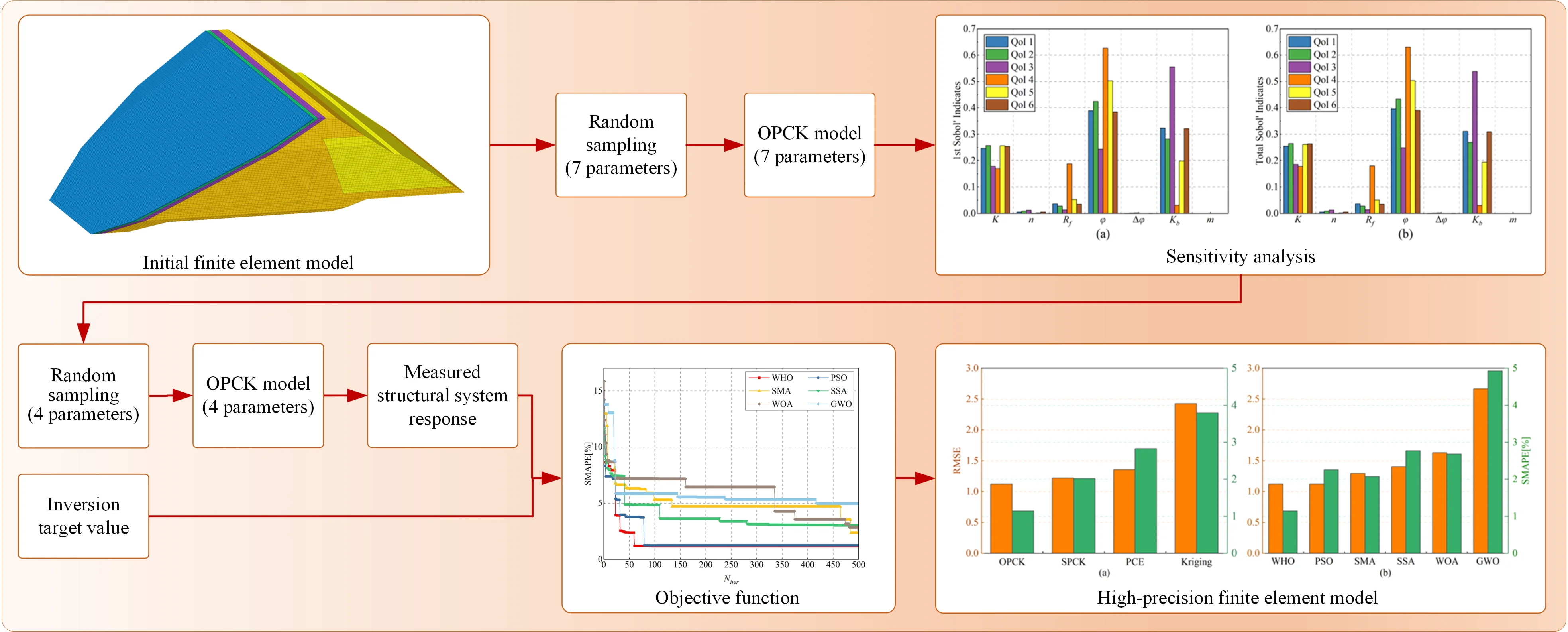
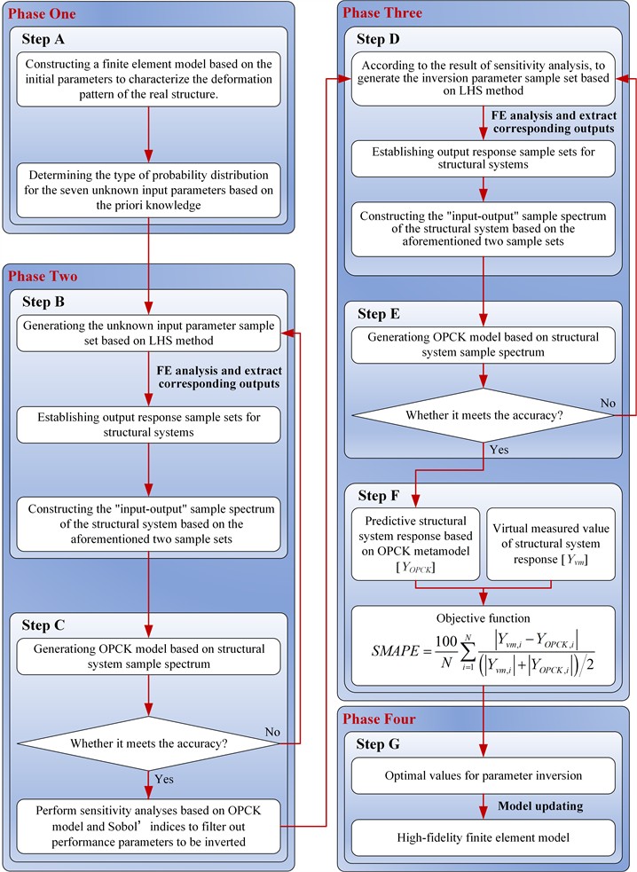
The proposed WHO_OPCK method for parameter inversion is structured in four phases. Initially, a FE model is established using benchmark parameters to simulate the settlement behavior of a real structure, accounting for uncertainties through a probabilistic model. Following this, a sensitivity analysis is conducted using a surrogate model to identify critical parameters. The surrogate model is then combined with the WHO algorithm to minimize an objective function, ultimately refining the parameter inversion for accurate model updates. The framework of the WHO_OPCK method is illustrated in Fig. 1.
3.2. Procedure of WHO_OPCK
The procedure of implementing the WHO_OPCK method is detailed below.
Phase One – Define the problem (Step A): The first step is to establish a FE model using benchmark parameters to characterize the settlement behavior of the real structure. It is necessary to define a prior probabilistic model for the unknown parameters to be determined inversely, including distribution type, mean, and deviation. Since real structure parameters are often random, incorporating uncertainty in the input parameters is more realistic.
Phase Two – Parameter sensitivity analysis based on surrogate modeling (Step B~C): Create a few input parameter datasets randomly using Latin Hypercube Sampling (LHS) method. Perform Finite Element Analysis (FEA) and extract the corresponding output response dataset. Construct the OPCK model from the “input-output” data and assess its accuracy with Leave-One-Out (LOO) cross-validation error. If the accuracy is satisfied, perform a parameter sensitivity analysis based on the Sobol’ indices and the constructed OPCK model to filter out performance parameters to be inverted; If the accuracy is insufficient, generate additional sampling points.
Phase Three – Coupling the OPCK model with WHO and minimizing the objective function (Step D~F): According to the results of the sensitivity analysis, a certain number of inversion parameter datasets are randomly generated using LHS method. Subsequently, the FEA is executed, and the output response dataset is extracted. Then, the same method as in step C is used to construct the OPCK model and evaluate its accuracy. Once an accurate OPCK model is established, it can replace the FE model for calculating structural responses, bypassing the high computational cost of FE model. Finally, the OPCK model is coupled with the WHO algorithm by integrating the predicted and target (virtual measured) outputs into an objective function.
Phase Four – Parameter inversion post-validation (Step G): The optimal values from the parameter inversion are processed and used as actual input parameters to update the FE model.
The symmetric mean absolute percentage error (SMAPE) is a common metric employed in statistics for evaluating prediction accuracy. Unlike Root Mean Square Error (RMSE), it is expressed as absolute percentages, making it easier to interpret. In this paper, SMAPE is chosen as the objective function to access the accuracy of the WHO_OPCK method. The formula is as follows:
where is the virtual measured value, is the predicted value from the OPCK model, and is the number of fitted points.
4. Nonlinear numerical modeling of CFRD
The WHO_OPCK method is applied to a multivariate nonlinear complex structure, the ZJTT CFRD, to explore the applicability of the proposed method to large hydraulic structures.
4.1. Description of ZJTT CFRD
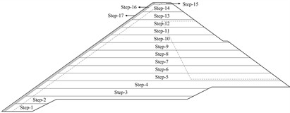
The ZJTT CFRD is the dam of the lower reservoir of a pumped storage power station. As illustrated in Fig. 2(a), it has a crest elevation of 209 m, a base elevation of 138 m, a maximum height of 71 m, and a total crest length of 404.25 m. The thickness of the concrete face slab is given by 0.4 + 0.003, where is the height from the calculated section to the top of the face slab, with a slope of 1:1.405. This study focuses on the period immediately following the completion of dam construction. During this period, the dam’s loading is predominantly influenced by its self-weight. As shown in Fig. 2(b-d), the displacement of the measurement point is used as the QoIs.
4.2. Simulation process
The layered stacking process of the rockfill dam was simulated using Abaqus, incorporating the Duncan E-B UMAT subroutine, developed in Fortran [21], for the rockfill material. Goodman contact elements with zero thickness were used to model the contact between the concrete face slabs and the bedding layer [28]. A three-dimensional numerical model was constructed to determine the displacement and stress distribution patterns of the dam body during the layered construction of the rockfill, as well as the stress-strain distribution patterns of the concrete face slab during the same period.
Fig. 1Framework to describe the WHO_OPCK method
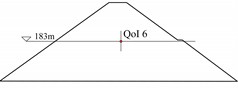
The material zoning consists of five parts: main rockfill, secondary rockfill, transition, cushion, and concrete face slab, as shown in Fig. 3(a). The main rockfill, secondary rockfill, transition and cushion layers were modeled using Duncan E-B model with the material parameters listed in Table 1. The concrete face slab was modeled with linear elasticity and the material parameters are shown in Table 2. The Goodman contact element parameters in Table 3 reflect the friction and stiffness of the contact surface, ensuring reliable simulation results.
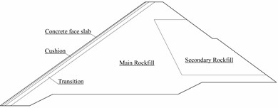
The stacking process was simulated using Abaqus life and death units, with the rock mass stacking divided into 15 steps, one step each for the cushion layer and the concrete face slab, as shown in Fig. 3(b).
Fig. 2Dam size and measurement profiles: a) longitudinal view of the dam, showing the profile locations where measurement points are distributed; b) cross-section at y= 361.99 m, showing the measurement point for Quantity of Interest QoI 1; c) cross-section at y= 229.99 m, showing the measurement points for QoIs 2, 3, 4, and 5; d) cross-section at y= 88.99 m, showing the measurement point for QoI 6
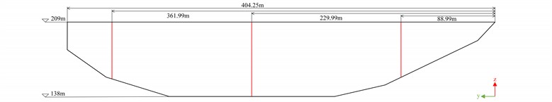
a) Longitudinal view of the dam
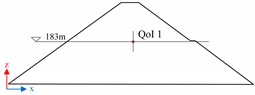
b) Cross-section at 361.99 m
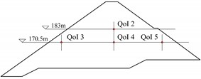
c) Cross-section at 229.99 m
d) Cross-section at 88.99 m
Table 1Nonlinear material parameters
Material | |||||||||||
Cushion | 1117.6 | 0.31 | 0.54 | 0.01 | 59 | 12.5 | 998.7 | 0.14 | 1900 | 0.31 | 2240 |
Transition | 1518.8 | 0.27 | 0.59 | 0.01 | 60.4 | 13.3 | 1039.4 | 0.06 | 1700 | 0.27 | 2210 |
Main rockfill | 1457.3 | 0.29 | 0.62 | 0.01 | 59.5 | 13.3 | 1028.5 | 0.04 | 2100 | 0.29 | 2220 |
Secondary rockfill | 1139.7 | 0.29 | 0.59 | 0.01 | 56.1 | 12.2 | 633.5 | 0.15 | 2000 | 0.29 | 2190 |
Note: the rockfill is a discrete material cohesion is 0, in order to numerical calculation convergence take 0.01 | |||||||||||
Table 2Linear material parameters
Elasticity () | Poisson’s ratio () | |
Concrete face slab | 28 GPa | 0.31 |
Table 3Goodman nonlinear contact parameters
Goodman | 4800 | 4800 | 0.56 | 0.74 | 36.6 |
Fig. 3ZJTT CFRD: a) Material zoning layout of the dam, showing the distribution and classification of different materials used in the construction; b) Layered construction process of the dam, illustrating the sequence and method by which the dam is built layer by layer
a) Material zoning
b) Layered construction process
Given that the dam is still under construction, the measured data could not be obtained. To demonstrate the efficiency of the proposed WHO_OPCK method in engineering applications, a “hypothesis testing” strategy was employed to verify the method’s feasibility. First, the LHS method was used to randomly generate 20 sets of material parameters for the CFRD model. The corresponding displacements at the measurement points were then calculated and averaged based on FEA. To account for the discrepancies between numerical simulations and real-world measurements, 20 % Gaussian noise was introduced into the mean values. Finally, one set of noise-containing data was randomly selected as the virtual measurement data, as described in Step F in Fig. 1.
5. Multi-parameter inversion of ZJTT CFRD
Parameter sensitivity analysis is essential before multi-parameter inversion. It helps identify how input parameters affect outputs and highlights the most influential parameters. This enables the optimization of key parameters while minimizing the impact of less critical factors in the inversion process.
5.1. Parameter sensitivity analysis
5.1.1. Parameter distribution space for sensitivity analysis
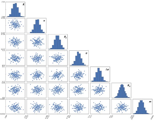
In this study, seven key parameters – elastic modulus coefficient , elastic modulus index , damage ratio , initial internal friction angle , rate of change of internal friction angle , bulk modulus coefficient , and bulk modulus index , are treated as unknown inputs. These parameters are assumed to follow a Gaussian distribution, with mean values based on average triaxial test results and a standard deviation set at 5 %.
A total of 140 samples were randomly selected using Latin Hypercube Sampling (LHS), as shown in Fig. 4. The probabilistic distribution models for the main rockfill parameters are provided in Table 4. For other zonal material parameters, raw data were used, so the inverse analysis focused solely on the main rockfill material parameters. The same method can be applied to invert other zonal material parameters, though this is not addressed in this work.
Table 4Distribution model of the unknown parameters for the Duncan E-B constitutive model of the main rockfill
Parameter | Symbol | Quantity | Bound |
Elastic modulus coefficient | N(1457.3,72.865) | [1165.84, 1748.76] | |
Elastic modulus index | N(0.29,0.0145) | [0.232, 0.348] | |
Failure ratio | N(0.62,0.031) | [0.496, 0.744] | |
Cohesion | 0.01 | – | |
Initial friction angle | N(59.5,2.975) | [47.6, 71.4] | |
Rate of change of internal friction angle | N(13.3,0.665) | [10.64, 15.96] | |
Bulk modulus coefficient | N(1028.5,51.425) | [822.8, 1234.2] | |
Bulk modulus index | N(0.04,0.002) | [0.032, 0.048] | |
Unloading modulus coefficient | 2100 | – | |
Unloading modulus index | 0.29 | – | |
Density | 2220 | – |
5.1.2. Construction of the surrogate model
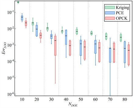
This section explores how the number of experimental designs () affects model accuracy and compares the OPCK surrogate model with classical PCE and Kriging. Surrogate models were built using varying to determine the optimal values for the OPCK model. A total of 140 initial samples were taken for the unknown parameters using LHS. Corresponding response output (QoI 1~6) was calculated. Then, surrogate models with different sizes of (i.e., 10, 20, 30, 40, 50, 60, 70, and 80) were constructed, this yielded 24 surrogate models. The for the six output responses in each case are shown in Fig. 5.
Fig. 4Seven-parameter random sampling results
From Fig. 5 the following results can be derived:
1) All three surrogate models show high accuracy across varying . ut Kriging has lower accuracy and greater discrepancies compared to PCE and OPCK. The OPCK model outperforms PCE in accuracy.
2) For the PCE model, decreases significantly from 10 to 40, then plateaus, showing no further improvement. In the OPCK model, the reduction is more pronounced between 10 and 40, after which accuracy stabilizes for 40.
3) While Kriging’s decreases with increasing , it doesn’t reach the desired accuracy (below 5 %) until 80.
Fig. 5The impact of the number of experimental designs (NDOE) on output accuracy and a comparison of three surrogate models
5.1.3. Sensitivity analysis
The Sobol’ index method, based on variance decomposition, determines the sensitivity of input variables by calculating their contribution to the total output variance [49]. In this study, the ErrLOO of the OPCK model is less than 10-2 when 50, meeting the predictive accuracy requirements for large hydraulic structures. Hence, parameter sensitivity analyses were conducted using the OPCK model instead of the computationally expensive ZJTT CFRD model. The sensitivity analysis results, considering the impact of the seven unknown input parameters on the ZJTT CFRD model’s output, are shown in Fig. 6. Key observations include:
1) , , , and exhibit high sensitivity in various QoI metrics, with and being particularly influential. These parameters are crucial in CFRD deformation and should be prioritized for calibration and optimization.
2) In contrast, , , and show low sensitivity and weak effects on QoI metrics, contributing minimally to CFRD deformation and are of secondary importance.
3) Sensitivities of QoI indicators to the same parameter vary. For example, is significant in QoI 4 and 5, while is prominent in QoI 6, reflecting the system’s nonlinear response. Multidimensional indicators should be considered in parameter analysis.
Fig. 6Results of parameter sensitivity analysis based on the OPCK model
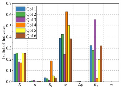
a) First-order Sobol’ indices
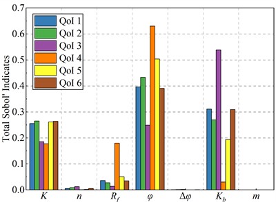
b) Total Sobol’ indices
The sensitivity analysis revealed that , , and are crucial for CFRD. The next step is multi-parameter inversion for these parameters to improve model accuracy and prediction.
5.2. Multi-parameter inversion
After the sensitivity analysis, , , , and were identified as key parameters. We will now perform a multi-parameter inversion to calibrate the model and match the virtual measured data.
Section 5.1.2 discussed key factors influencing surrogate model accuracy. This section focuses on the impact of the number of search individuals () in the WHO_OPCK method, with Niter set to 500. Results are shown in Fig. 7, and observations are as follows:
1) Fig. 7(a) shows that as increases, convergence speed improves, particularly for 50, where the error decreases rapidly. Smaller values (e.g., 30 or 35) lead to slower convergence, especially at the start, due to limited search space exploration.
2) The SMAPE value shows significant variation at lower , dropping sharply at 35 and 40. For 40, SMAPE stabilizes, indicating improved convergence accuracy as more individuals help find the global optimum.
3) Fig. 7(b) shows that computation time increases with , as more individuals require processing more data. The increase stabilizes at 60, where time overhead is moderate and accuracy remains high, offering an optimal balance.
Based on the results, surrogate models and inversion methods with 50 and 60 were chosen for comparison.
For the computationally expensive 3D CFRD, using 50 for the surrogate model results in a total computation time of about 28 hours (0.56 hours per run) in ABAQUS. In contrast, the traditional WHO algorithm with direct FE model calls for iterative inversion would take approximately 16,800 hours (0.56×60×500) for 60 and 500. This immense computational demand makes the traditional method impractical for 3D CFRD parameter inversion, limiting its real-world engineering application.
Fig. 7The effect of different N on the accuracy of WHO_OPCK method
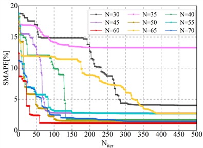
a) Convergence properties
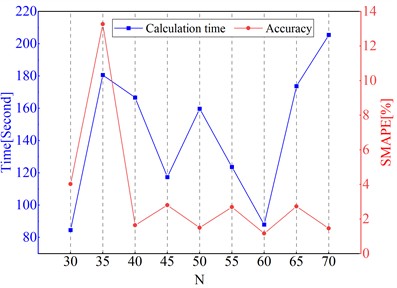
b) Computational time and convergence accuracy
The WHO optimization algorithm was combined with various surrogate models to compare the convergence of WHO_OPCK with WHO_SPCK, WHO_PCE, and WHO_Kriging. Fig. 8 shows the convergence speeds, accuracies, and computation times, while Table 5 presents the inversion results. The following conclusions can be drawn:
1) WHO_OPCK achieves faster convergence and greater robustness in parameter inversion. It outperforms other methods, especially WHO_SPCK and WHO_Kriging, by finding better solutions in fewer iterations while maintaining stability.
2) WHO_OPCK provides more accurate inversion results than WHO_SPCK, WHO_PCE, and WHO_Kriging, demonstrating superior convergence accuracy.
3) WHO_OPCK, though slightly slower than WHO_PCE, outperforms WHO_SPCK and WHO_Kriging in efficiency, requiring only 46 % and 16.8 % of their respective computation times, achieving an optimal balance between time and accuracy.
By combining the strengths of PCE and Kriging, WHO_OPCK excels in both accuracy and speed while keeping computation time reasonable, offering better cost-effectiveness in practical applications.
Table 5The results of parameter inversion based on WHO combined with different surrogate models
Method | ||||
WHO_OPCK | 1594.123 | 0.713 | 64.577 | 933.344 |
WHO_SPCK | 1550.424 | 0.609 | 59.377 | 976.841 |
WHO_PCE | 1437.214 | 0.562 | 59.270 | 1028.357 |
WHO_Kriging | 1426.354 | 0.718 | 65.613 | 953.810 |
Meanwhile, we also coupled OPCK with classical optimization algorithms (PSO, SMA, SSA, WOA, GWO) [11, 12, 50-52] to compare convergence and computational efficiency. Fig. 9 shows the convergence speed, accuracy, and computation time, while Table 6 presents the inversion parameter results. The following conclusions can be drawn:
1) WHO_OPCK outperforms OPCK with classical algorithms in both convergence speed and accuracy, showing strong performance in complex CFRD optimization.
2) Fig. 9(b) shows that parameter inversion accuracy and convergence speed do not directly correlate with inversion time. Despite its high computation load, SSA does not achieve the highest accuracy, while WOA, with the second-highest time, has the lowest accuracy.
3) WHO_OPCK achieves the highest accuracy and shortest inversion time, making it the most efficient and effective method among the comparisons.
Fig. 8Comparison of WHO combined with different surrogate models
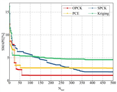
a) Convergence properties and accuracy
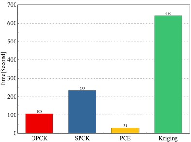
b) Computation time
Table 6The results of parameter inversion based on different optimization algorithms combined with OPCK
Method | ||||
WHO_OPCK | 1594.123 | 0.713 | 64.577 | 933.344 |
PSO_OPCK | 1311.315 | 0.527 | 68.425 | 1001.838 |
SMA_OPCK | 1663.778 | 0.672 | 61.071 | 927.500 |
SSA_OPCK | 1675.895 | 0.639 | 56.853 | 996.650 |
WOA_OPCK | 1524.948 | 0.622 | 60.770 | 960.481 |
GWO_OPCK | 1550.042 | 0.571 | 60.778 | 981.066 |
Fig. 9Comparison of different optimization algorithms combined with OPCK
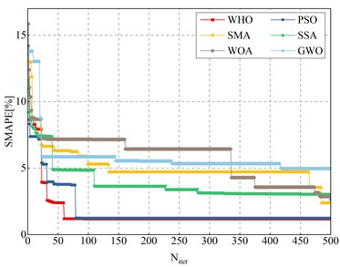
a) Convergence characteristics and accuracy
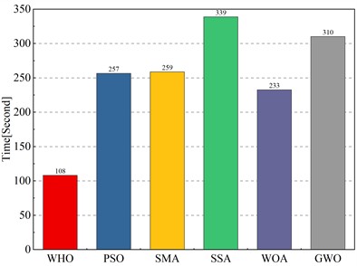
b) Computation time
The parameter inversion results are used to update the FE model, which is then simulated with the new parameters. The output is compared to the virtual measured values, with errors assessed using RMSE and SMAPE. The detailed output and error results are shown in Table 7 and 8, and Fig. 10 provides a visual comparison. The following conclusions can be drawn:
1) Fig. 10(a) shows that the FE model updated with WHO_OPCK achieves higher accuracy, with significant advantages in both RMSE and SMAPE. Among the surrogate models, WHO_Kriging has the greatest error and lowest accuracy.
2) Fig. 10(b) shows that the FE model updated with WHO_OPCK has better accuracy. SMA and WHO show similar errors, while WOA performs the worst, with the largest error and lowest accuracy.
Table 7Comparison of predicted and virtual measured values of WHO combined with different surrogate models
Condition | QoIs | Virtual measured value (mm) | OPCK | SPCK | PCE | Kriging |
Deformation | 1 | 95.90 | 95.75 | 96.89 | 96.60 | 98.52 |
2 | 121.44 | 119.35 | 122.07 | 122.03 | 123.18 | |
3 | 32.56 | 32.53 | 32.35 | 33.83 | 34.75 | |
4 | 102.18 | 103.75 | 103.99 | 102.82 | 105.74 | |
5 | 24.81 | 25.65 | 26.72 | 27.63 | 26.42 | |
6 | 94.46 | 94.41 | 95.23 | 95.00 | 96.82 | |
RMSE | 1.122 | 1.218 | 1.358 | 2.428 | ||
SMAPE | 1.147 % | 2.021 % | 2.828 % | 3.793 % |
Table 8Comparison of predicted and virtual measured values of different optimization algorithms combined with OPCK
Condition | QoIs | Virtual measured value (mm) | WHO | PSO | SMA | SSA | WOA | GWO |
Deformation | 1 | 95.90 | 95.75 | 96.29 | 96.28 | 96.06 | 97.38 | 94.78 |
2 | 121.44 | 119.35 | 120.86 | 120.81 | 121.04 | 122.57 | 119.66 | |
3 | 32.56 | 32.53 | 34.73 | 31.27 | 35.36 | 31.56 | 26.67 | |
4 | 102.18 | 103.75 | 102.91 | 104.68 | 102.64 | 104.84 | 102.21 | |
5 | 24.81 | 25.65 | 26.14 | 25.93 | 26.70 | 26.52 | 26.26 | |
6 | 94.46 | 94.41 | 94.76 | 95.09 | 94.37 | 95.73 | 93.21 | |
RMSE | 1.122 | 1.123 | 1.295 | 1.406 | 1.633 | 2.669 | ||
SMAPE | 1.147 % | 2.260 % | 2.072 % | 2.774 % | 2.684 % | 4.926 % |
Fig. 10Comparison of FEA errors based on inversion results and virtual measured data
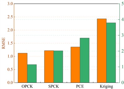
a) WHO combined with different surrogate models
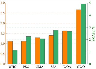
b) Different optimization algorithms combined with OPCK
6. Conclusions
Assessing CFRD deformation is challenging due to the complex construction process and large volume of discrete rockfill material, yet it is crucial for safe operation.
Existing CFRD parameter inversion relies on pure optimization, directly invoking time-consuming FE models, which limits efficiency and accuracy. This creates a challenge in balancing computational efficiency with accuracy. Consequently, most of these methods are restricted to parameter inversion for 2D CFRDs, with few studies addressing the complex and time-consuming task of high-precision, high-efficiency parameter inversion for 3D CFRDs.
This work develops the efficient OPCK surrogate model for 3D CFRD inversion, combined with the WHO algorithm to create WHO_OPCK, enabling fast and accurate parameter inversion. Some conclusions are summarized below:
1) For the WHO optimization algorithm, the number of search individuals N significantly impacts its search performance, thereby affecting the accuracy of WHO_OPCK. This feature can be generalized to other research applications of population-based optimization algorithms.
2) OPCK offers significant advantages in terms of computational cost, with low requirements, high efficiency, and minimal resource consumption. This makes WHO_OPCK not only accurate but also highly suitable for large-scale optimization problems where computational efficiency is essential.
3) Taking the 3D CFRD as an example, traditional pure optimization approaches are unable to identify its parameters. In contrast, the proposed WHO_OPCK method successfully determines these parameters, offering a feasible solution for fast parameter inversion of the 3D CFRD.
4) Compared to existing representative parameter inversion methods, including WHO_SPCK, WHO_PCE, WHO_Kriging, PSO_OPCK, SMA_OPCK, SSA_OPCK, WOA_OPCK, and GWO_OPCK, the proposed WHO_OPCK method demonstrates superior accuracy and efficiency in dam parameter inversion. This makes it a more effective and reliable approach for tackling the challenges posed by complex dam models.
Although the proposed WHO_OPCK method has unrivalled efficiency advantages over traditional methods, it still has some limitations that need to be considered:
1) Due to the classical “curse of dimensionality”, the predictive performance of surrogate model in a high-dimensional parameter space will be notably reduced. Hence, the sample size for constructing the surrogate model can be increased appropriately based on the complexity of the problem.
2) Surrogate models offer efficient approximate computations, their overall computational efficiency still depends significantly on the forward computation models (such as FE models). In other words, generating the initial dataset typically consumes most of the time spent constructing the surrogate model.
3) The number of design experiments () used to construct the surrogate models is typically not known in advance, necessitating the construction of surrogate models using different sizes of for comparison.
References
-
A. Karimi, S. L. Heydari, F. Kouchakmohseni, and M. Naghiloo, “Scheduling and value of pumped storage hydropower plant in Iran power grid based on fuel-saving in thermal units,” Journal of Energy Storage, Vol. 24, p. 100753, Aug. 2019, https://doi.org/10.1016/j.est.2019.04.027
-
Y. Kong, Z. Kong, Z. Liu, C. Wei, J. Zhang, and G. An, “Pumped storage power stations in China: The past, the present, and the future,” Renewable and Sustainable Energy Reviews, Vol. 71, pp. 720–731, May 2017, https://doi.org/10.1016/j.rser.2016.12.100
-
X. Luo, J. Wang, M. Dooner, and J. Clarke, “Overview of current development in electrical energy storage technologies and the application potential in power system operation,” Applied Energy, Vol. 137, pp. 511–536, Jan. 2015, https://doi.org/10.1016/j.apenergy.2014.09.081
-
C. Schwarzbach and E. Haber, “Finite element based inversion for time-harmonic electromagnetic problems,” Geophysical Journal International, Vol. 193, No. 2, pp. 615–634, May 2013, https://doi.org/10.1093/gji/ggt006
-
P. Broumand, “Inverse problem techniques for multiple crack detection in 2D elastic continua based on extended finite element concepts,” Inverse Problems in Science and Engineering, Vol. 29, No. 12, pp. 1702–1728, Dec. 2021, https://doi.org/10.1080/17415977.2021.1872564
-
S. Niu, Y. Zhao, and H. Bao, “Shape sensing of plate structures through coupling inverse finite element method and scaled boundary element analysis,” Measurement, Vol. 190, p. 110676, Feb. 2022, https://doi.org/10.1016/j.measurement.2021.110676
-
B. T. Johansson, D. Lesnic, and T. Reeve, “A meshless method for an inverse two-phase one-dimensional linear Stefan problem,” Inverse Problems in Science and Engineering, Vol. 21, No. 1, pp. 17–33, Jan. 2013, https://doi.org/10.1080/17415977.2012.665906
-
J. H. Deng and C. F. Lee, “Displacement back analysis for a steep slope at the three gorges project site,” International Journal of Rock Mechanics and Mining Sciences, Vol. 38, No. 2, pp. 259–268, Feb. 2001, https://doi.org/10.1016/s1365-1609(00)00077-0
-
S. P. Neuman, G. E. Fogg, and E. A. Jacobson, “A statistical approach to the inverse problem of aquifer hydrology: 2. Case study,” Water Resources Research, Vol. 16, No. 1, pp. 33–58, Jul. 2010, https://doi.org/10.1029/wr016i001p00033
-
S. W. Alves and J. F. Hall, “System identification of a concrete arch dam and calibration of its finite element model,” Earthquake Engineering and Structural Dynamics, Vol. 35, No. 11, pp. 1321–1337, Apr. 2006, https://doi.org/10.1002/eqe.575
-
J. Kennedy and R. Eberhart, “Particle swarm optimization,” in ICNN’95 – International Conference on Neural Networks, Vol. 4, pp. 1942–1948, Jul. 2025, https://doi.org/10.1109/icnn.1995.488968
-
S. Mirjalili and A. Lewis, “The whale optimization algorithm,” Advances in Engineering Software, Vol. 95, pp. 51–67, May 2016, https://doi.org/10.1016/j.advengsoft.2016.01.008
-
J. Tsitsiklis, D. Bertsekas, and M. Athans, “Distributed asynchronous deterministic and stochastic gradient optimization algorithms,” IEEE Transactions on Automatic Control, Vol. 31, No. 9, pp. 803–812, Sep. 1986, https://doi.org/10.1109/tac.1986.1104412
-
S. Razavi, B. A. Tolson, and D. H. Burn, “Review of surrogate modeling in water resources,” Water Resources Research, Vol. 48, No. 7, Jul. 2012, https://doi.org/10.1029/2011wr011527
-
L. Yifei, C. Maosen, H. Tran-Ngoc, S. Khatir, and M. Abdel Wahab, “Multi-parameter identification of concrete dam using polynomial chaos expansion and slime mould algorithm,” Computers and Structures, Vol. 281, p. 107018, Jun. 2023, https://doi.org/10.1016/j.compstruc.2023.107018
-
Y. Li, M. A. Hariri-Ardebili, T. Deng, Q. Wei, and M. Cao, “A surrogate-assisted stochastic optimization inversion algorithm: Parameter identification of dams,” Advanced Engineering Informatics, Vol. 55, p. 101853, Jan. 2023, https://doi.org/10.1016/j.aei.2022.101853
-
J. P. C. Kleijnen, “Kriging metamodeling in simulation: A review,” European Journal of Operational Research, Vol. 192, No. 3, pp. 707–716, Feb. 2009, https://doi.org/10.1016/j.ejor.2007.10.013
-
C. Wang, Y. Li, N. H. Tran, D. Wang, S. Khatir, and M. A. Wahab, “Artificial neural network combined with damage parameters to predict fretting fatigue crack initiation lifetime,” Tribology International, Vol. 175, p. 107854, Nov. 2022, https://doi.org/10.1016/j.triboint.2022.107854
-
R. Ghanem, G. Saad, and A. Doostan, “Efficient solution of stochastic systems: application to the embankment dam problem,” Structural Safety, Vol. 29, No. 3, pp. 238–251, Jul. 2007, https://doi.org/10.1016/j.strusafe.2006.07.015
-
L. Yifei et al., “Structure damage identification in dams using sparse polynomial chaos expansion combined with hybrid K-means clustering optimizer and genetic algorithm,” Engineering Structures, Vol. 283, p. 115891, May 2023, https://doi.org/10.1016/j.engstruct.2023.115891
-
G. Shahzadi and A. Soulaïmani, “Deep neural network and polynomial chaos expansion-based surrogate models for sensitivity and uncertainty propagation: an application to a rockfill dam,” Water, Vol. 13, No. 13, p. 1830, Jun. 2021, https://doi.org/10.3390/w13131830
-
M. Hariri-Ardebili, G. Mahdavi, A. Abdollahi, and A. Amini, “An RF-PCE hybrid surrogate model for sensitivity analysis of dams,” Water, Vol. 13, No. 3, p. 302, Jan. 2021, https://doi.org/10.3390/w13030302
-
X. Guo and D. Dias, “Kriging based reliability and sensitivity analysis – application to the stability of an earth dam,” Computers and Geotechnics, Vol. 120, p. 103411, Apr. 2020, https://doi.org/10.1016/j.compgeo.2019.103411
-
Y. Wang, Y. Liu, and X. Ma, “Updated kriging-assisted shape optimization of a gravity dam,” Water, Vol. 13, No. 1, p. 87, Jan. 2021, https://doi.org/10.3390/w13010087
-
A. Abdollahi, A. Amini, and M. A. Hariri-Ardebili, “An uncertainty-aware dynamic shape optimization framework: Gravity dam design,” Reliability Engineering and System Safety, Vol. 222, p. 108402, Jun. 2022, https://doi.org/10.1016/j.ress.2022.108402
-
A. Amini, A. Abdollahi, M. A. Hariri-Ardebili, and U. Lall, “Copula-based reliability and sensitivity analysis of aging dams: Adaptive Kriging and polynomial chaos Kriging methods,” Applied Soft Computing, Vol. 109, p. 107524, Sep. 2021, https://doi.org/10.1016/j.asoc.2021.107524
-
V. H. Vu, M. Thomas, A. A. Lakis, and L. Marcouiller, “Operational modal analysis by updating autoregressive model,” Mechanical Systems and Signal Processing, Vol. 25, No. 3, pp. 1028–1044, Apr. 2011, https://doi.org/10.1016/j.ymssp.2010.08.014
-
P. Sun, T. Bao, C. Gu, M. Jiang, T. Wang, and Z. Shi, “Parameter sensitivity and inversion analysis of a concrete faced rock-fill dam based on HS-BPNN algorithm,” Science China Technological Sciences, Vol. 59, No. 9, pp. 1442–1451, Aug. 2016, https://doi.org/10.1007/s11431-016-0213-y
-
B. Liu, H. Li, G. Wang, W. Huang, P. Wu, and Y. Li, “Dynamic material parameter inversion of high arch dam under discharge excitation based on the modal parameters and Bayesian optimised deep learning,” Advanced Engineering Informatics, Vol. 56, p. 102016, Apr. 2023, https://doi.org/10.1016/j.aei.2023.102016
-
J. Li, C. Chen, Z. Wu, and J. Chen, “Multi-source data-driven unsaturated seepage parameter inversion: Application to a high core rockfill dam,” Journal of Hydrology, Vol. 617, p. 129171, Feb. 2023, https://doi.org/10.1016/j.jhydrol.2023.129171
-
L. Yifei et al., “Metamodel-assisted hybrid optimization strategy for model updating using vibration response data,” Advances in Engineering Software, Vol. 185, p. 103515, Nov. 2023, https://doi.org/10.1016/j.advengsoft.2023.103515
-
S. Pan, T. Li, G. Shi, Z. Cui, H. Zhang, and L. Yuan, “The inversion analysis and material parameter optimization of a high earth-rockfill dam during construction periods,” Applied Sciences, Vol. 12, No. 10, p. 4991, May 2022, https://doi.org/10.3390/app12104991
-
Y. Li, H.-L. Minh, M. Cao, X. Qian, and M. Abdel Wahab, “An integrated surrogate model-driven and improved termite life cycle optimizer for damage identification in dams,” Mechanical Systems and Signal Processing, Vol. 208, p. 110986, Feb. 2024, https://doi.org/10.1016/j.ymssp.2023.110986
-
T. Bao, J. Li, Y. Lu, and C. Gu, “IDE-MLSSVR-based back analysis method for multiple mechanical parameters of concrete dams,” Journal of Structural Engineering, Vol. 146, No. 8, Aug. 2020, https://doi.org/10.1061/(asce)st.1943-541x.0002602
-
H. Li, G. Wang, B. Wei, Y. Zhong, and L. Zhan, “Dynamic inversion method for the material parameters of a high arch dam and its foundation,” Applied Mathematical Modelling, Vol. 71, pp. 60–76, Jul. 2019, https://doi.org/10.1016/j.apm.2019.02.008
-
G. Blatman, “Adaptive sparse polynomial chaos expansions for uncertainty propagation and sensitivity analysis,” Université Blaise Pascal, 2009.
-
N. Fajraoui, S. Marelli, and B. Sudret, “Sequential design of experiment for sparse polynomial chaos expansions,” SIAM/ASA Journal on Uncertainty Quantification, Vol. 5, No. 1, pp. 1061–1085, Jan. 2017, https://doi.org/10.1137/16m1103488
-
M. Stone, “Cross-validatory choice and assessment of statistical predictions,” Journal of the Royal Statistical Society Series B: Statistical Methodology, Vol. 36, No. 2, pp. 111–133, Jan. 1974, https://doi.org/10.1111/j.2517-6161.1974.tb00994.x
-
S. Geisser, “The predictive sample reuse method with applications,” Journal of the American Statistical Association, Vol. 70, No. 350, pp. 320–328, Jun. 1975, https://doi.org/10.1080/01621459.1975.10479865
-
T. J. Santner, B. J. Williams, and W. I. Notz, The Design and Analysis of Computer Experiments. New York, NY: Springer New York, 2003.
-
R. Schobi, B. Sudret, and J. Wiart, “Polynomial-chaos-based kriging,” International Journal for Uncertainty Quantification, Vol. 5, No. 2, pp. 171–193, Jan. 2015, https://doi.org/10.1615/int.j.uncertaintyquantification.2015012467
-
R. Schöbi, B. Sudret, and S. Marelli, “Rare event estimation using polynomial-chaos kriging,” ASCE-ASME Journal of Risk and Uncertainty in Engineering Systems, Part A: Civil Engineering, Vol. 3, No. 2, Jun. 2017, https://doi.org/10.1061/ajrua6.0000870
-
P. Kersaudy, B. Sudret, N. Varsier, O. Picon, and J. Wiart, “A new surrogate modeling technique combining Kriging and polynomial chaos expansions – Application to uncertainty analysis in computational dosimetry,” Journal of Computational Physics, Vol. 286, pp. 103–117, Apr. 2015, https://doi.org/10.1016/j.jcp.2015.01.034
-
B. Efron and T. Hastie, “Johnstone I, et al. Least angle regression,” Annals of Statistics, Vol. 32, No. 2, pp. 407–499, 2004.
-
G. Blatman and B. Sudret, “Adaptive sparse polynomial chaos expansion based on least angle regression,” Journal of Computational Physics, Vol. 230, No. 6, pp. 2345–2367, Mar. 2011, https://doi.org/10.1016/j.jcp.2010.12.021
-
G. Blatman and B. Sudret, “An adaptive algorithm to build up sparse polynomial chaos expansions for stochastic finite element analysis,” Probabilistic Engineering Mechanics, Vol. 25, No. 2, pp. 183–197, Apr. 2010, https://doi.org/10.1016/j.probengmech.2009.10.003
-
G. Blatman and B. Sudret, “Sparse polynomial chaos expansions and adaptive stochastic finite elements using a regression approach,” Comptes Rendus. Mécanique, Vol. 336, No. 6, pp. 518–523, Apr. 2008, https://doi.org/10.1016/j.crme.2008.02.013
-
I. Naruei and F. Keynia, “Wild horse optimizer: a new meta-heuristic algorithm for solving engineering optimization problems,” Engineering with Computers, Vol. 38, No. S4, pp. 3025–3056, Jun. 2021, https://doi.org/10.1007/s00366-021-01438-z
-
J. Nossent, P. Elsen, and W. Bauwens, “Sobol’ sensitivity analysis of a complex environmental model,” Environmental Modelling and Software, Vol. 26, No. 12, pp. 1515–1525, Dec. 2011, https://doi.org/10.1016/j.envsoft.2011.08.010
-
S. Li, H. Chen, M. Wang, A. A. Heidari, and S. Mirjalili, “Slime mould algorithm: A new method for stochastic optimization,” Future Generation Computer Systems, Vol. 111, pp. 300–323, Oct. 2020, https://doi.org/10.1016/j.future.2020.03.055
-
J. Xue and B. Shen, “A novel swarm intelligence optimization approach: sparrow search algorithm,” Systems Science and Control Engineering, Vol. 8, No. 1, pp. 22–34, Jan. 2020, https://doi.org/10.1080/21642583.2019.1708830
-
S. Mirjalili, S. M. Mirjalili, and A. Lewis, “Grey wolf optimizer,” Advances in Engineering Software, Vol. 69, pp. 46–61, Mar. 2014, https://doi.org/10.1016/j.advengsoft.2013.12.007
About this article

The authors are grateful for the Jiangsu-Czech Bilateral Co-funding R&D Project (No. BZ2023011), and the Fundamental Research Funds for the Central Universities (No. B220204002).
The datasets generated during and/or analyzed during the current study are available from the corresponding author on reasonable request.
Liurui Li: investigation, methodology, visualization, writing - original draft preparation, data curation. Shuping Liu: supervision, writing-review and editing. Linna Li: resources, formal analysis. Fan Liu: investigation, validation, resources. Yifei Li: validation, software, writing-review and editing, supervision. Xin Zhang: writing-review and editing, resources, formal analysis. Maosen Cao: conceptualization, supervision, resources, funding acquisition, writing-review and editing.
