Performance assessment of network system network comprising four subsystems via multi failure and multi repair methodology

Sharma, Shailly; Singh, V. V.; Parihar, Priyavada; Neupane, Padam Lal

doi:10.21595/mme.2025.24893

Mathematical Models in Engineering

Browse Journal

Submit article

Published: 16 August 2025

Check for updates

Performance assessment of network system network comprising four subsystems via multi failure and multi repair methodology

Shailly Sharma¹

V. V. Singh²

Priyavada Parihar³

Padam Lal Neupane⁴

^{1, 3}Department of Mathematics Lingayas Vidyapeeth, Faridabad Haryana, India

²Department of Mathematics Noida International University, Greater Noida, India

⁴Department of Mathematics, Tribhuvan University, Nepal

Corresponding Author:

V. V. Singh

Cite the article Download PDF

Article in Press

Downloads 32

Abstract

A multi-dimensional repair approach is the most effective policy for restoring repairable systems. This research study analyzes a complex repairable system that consists of four subsystems with different configurations. The system consists of four subsystems: Subsystem 1 contains a single unit, Subsystem 2 includes n identical units operating under a k-out-of-n: G policy, Subsystem 3 features two identical load balancers responsible for distributing the load (with at least one required for operation), and Subsystem 4 consists of four identical units functioning under a 3-out-of-4: G policy. It is assumed that all subsystems have constant failure rates that are distributed exponentially. General repair, which is utilized while the system continues to function in accordance with the established operating policy, and copula-based repair, which is employed when the system stops completely, are the two types of repair techniques that are put into practice. A supplementary variable approach is incorporated to analyses system performance. Various reliability measures are computed using Maple 18, software, and future behaviour of system have been predicted in long run operation. By means of illustrations in the tables and graph it clearly shown how the copula repair is beneficial over ordinary repair.

1. Introduction

One defining feature of engineering systems is their artificial nature. The role of human intervention in such systems varies depending on their function and design. Engineering systems must be reliable; otherwise, they fail to serve their intended purpose. Many existing systems in production, communication, transportation, information technology, and computing are artificial and range in complexity from simple to highly complex. However, real-world system reliability can be significantly impacted by interdependent components (subsystems), primarily through shared stress, shared loads, or common-cause failures, see Barlow and F. Prochan, [1]. In system reliability analysis, the dependence concept of multivariate models for nonrepairable systems have been studied by many authors including. H. Joe [2]. Repairable systems are defined as those that can be fixed to work properly again after a failure, without needing to replace the whole thing. Repairable systems are commonly modeled using renewal processes for perfect repair and nonhomogeneous Poisson processes for minimal repair. The model of system failure is built from the failures of its components. A common simplification is to model systems and components as having only two possible states: functioning or non-functioning. This failure process is open to several interpretations. The reliability block diagram (success-oriented) and fault tree analysis (failure-oriented) are among these. The failures and repairs of models in system reliability follow different patterns. The models in which both failure and repairs follow constant and exponential distribution and constant repair distributions are usually analyzed by employing the Champman Kolmogorov method, however, the systems in which failures follow constant exponential distribution and repair follow variable distribution are analyses incorporating supplementary variable method D. R. Cox [3]. The repair follows different distributions as general distribution and copula distribution. In general repair distribution an ordinary repair facility is provided to the failed unit/ component/ subsystem. Due to normal efficiency of repair man, it takes more time to repair, and the system remains shutdown for the time during maintenance. Another type of repair distribution is exponential distribution which might be costly than normal repair. Whenever the system is in operational mode with some reduce efficiency, the general repair can be employed to restore the failed unit but if the system/ subsystem is in complete shutdown mode the copula distribution should be employed for quickly restore the failed system. Varies copula distribution are available in probabilistic theory literature and the Gumbel Hougaard family copula Nelson, R. B. Nelson [4] is one of the simple forms which couples general distribution and exponential distribution.

Numerous repairable systems have been analyzed in past research, including studies by, and Ashish Kumar and Malik [5], Dalah and Singh [6], Singh and Jyoti Gulati [7], and I. Yusuf and B. Yusuf [8]. These studies assume different types of failure and repair strategies. The Chapman-Kolmogorov differential equation typically analyzes the performance of a system following constant failure and repair rates in the available literature. However, when a system follows constant failure rates but incorporates variable multi-repair strategies, its performance is evaluated using the supplementary variable approach.

Authors such as Dalah and Singh [6] and Singh and Gulati [7] have employed the supplementary variable approach to analyze system performance. A system is a combination of components, parts, and subsystems that one can arrange in different configurations, including series, parallel, and mixed configurations. Among these, the k-out-of-n: G/F; system configuration is significant in industrial systems such as oil transfer networks, digital parking systems, and street lighting systems, where two fixed numbers ( $k$ and $n$ ) play a crucial role in determining system operation.

Several researchers have explored the k-out-of-n: G system configuration. A. Mishra and M. Jain [9] examine availability of k-out-of-n: F system with constant failure and general repair using supplementary variable approach. Four states were taken into consideration when Rawal et al. [10] examined the performance of networked systems: perfect, minor degraded, major degraded, and complete failure. K. G. Ramamurthy [11] have characterized the simple form of reliability functions of consecutive k-out-of-n: G system. Xiaolin et al. [12], studied a complex repairable system with two types of components: ordinary components and key components in which the repair was preference to key components failure over ordinary components. Rawal and Singh [13] studied a system with two subsystems operating under this configuration using joint probability distribution and a copula repair scheme. A genetic algorithm was used by Vijaykumar and Kumudini Devi [14] to suggest the best position for FACTS controllers in a multi-power machine system. Ibrahim Yusuf et al. [15] analyzed the cost-benefit aspects of mixed standby unit systems. Singh and Poonia [16] examined a two-subsystem series configuration by evaluating system reliability metrics under two repair strategies. Author P. K. Poonia [17] analyzed a system with computer lab of networking systems consisting of subsystems in a series configuration under various types of failure and multi repair using copula linguistic. When redundant units in the system are ready to take over the load of a failed unit, standard repair procedures may be used to repair the failed unit or component. Also in case of many industrial system where the system configuration of k-out-n:G/ F exits one can use the ordinary/general repair to restore the failed components till it approaches to minor partial failure or major partial failure but as the system bears the completely shut down mode it need fast repair hence the completely failed state need to be restore via incorporate the copula distribution. Although several copula distributions are available in the stochastic theory, the Gumbel Hougaard family copula is easy and approachable to use.

In order to assess multiple reliability measures, use of copula distribution, Dhruv Raghav et al. [18] investigated the performance of a k-out-of-n: G system utilizing two types of repair processes and multiple states failure modes. Ajay Kumar et al. [19] explored system performance under software upgrades and load recovery using Weibull distribution. Authors, H. I. Ayagi et. [20] assessed the performance of a complex system with three subsystems in series arrangement and a multi-repair technique. Monika Saini and Ashish Kumar [21] examined the operational production efficiency of a ghee production unit in a milk plant through RAMD (Reliability, Availability, Maintenance, and Dependability) analysis, employing the Markov process and the Kolmogorov differential equation method. Ibrahim Yusuf et al. [22] assessed the performance of mixed standby serial systems using a probabilistic approach with supplementary variables. A complex system under $k$ degraded states with non-identical load balance have been examined by V. V Singh et al. [23].

While recent publications exist, comparative studies are lacking. Ahmed T Alhasani et al. [24] conducted a collaborative study on diagnosing breast cancer using data mining, achieving 96 % accuracy, with precision (18.57 %) and recall (50 %) as weighted averages. The model’s results, benchmarked against similar research, reveal substantial advancements, suggesting new possibilities in breast cancer detection. Mahmoud E Mohamed [25] studied a review management technique for sustainable energy production. These results emphasize the critical part waste-to-power energy (WPE) plays in boosting energy efficiency, promoting cleaner production, and creating a robust financial framework. Recently, Khodadadi and associates explored an archive-based multi-objective arithmetic optimization algorithm to tackle industrial engineering challenges. To assess its effectiveness for real-world engineering problems, the method was evaluated using seven benchmark functions, ten CEC-2020 mathematical functions, and eight constrained engineering design problems. The study by Hobiny, Abbas, and Marin [26] examines the impact of hyperbolic two-temperature theory on wave propagation within a semiconductor material featuring a spherical cavity. El-Sayed et al. [27] investigated the particle swarm optimization algorithm, a nature-inspired optimization technique. Meta-heuristic algorithms, inspired by nature, use biological evolution to develop powerful, innovative algorithms.

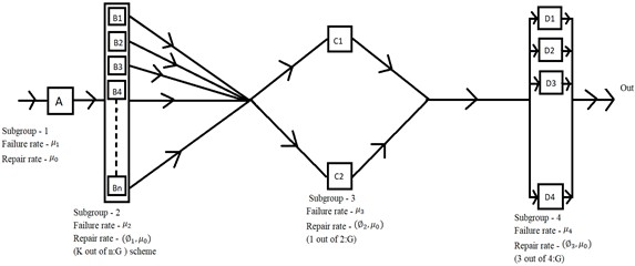
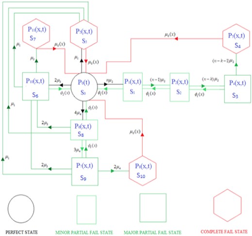
Fig. 1a) System architecture, and b) state transition diagram

a)

b)

Although extensive research has been conducted by the authors, very few studies have analyzed the performance of mixed k-out-of-n: G systems using the supplemental variable approach in conjunction with copula-based repair. In the present study, we focus on analyzing a system comprising four subsystems arranged in a series configuration:

1) Subsystem 1 consists of a single independent unit.

2) Subsystem 2 includes parallel units working under the k-out-of-n: G policy.

3) Subsystem 3 features two identical load balancers that distribute the load from Subsystem 2; at least one balancer must be operational for proper functioning.

4) Subsystem 4 consists of four identical units operating in parallel under the 3-out-of-4: G working policy.

Using probabilistic theoretical arguments, we define eleven possible states $(S_{0}, S_{1}, S_{2}, \dots, S_{10})$ , representing the system’s perfectly operational state $S_{0}$ , minor degraded states $S_{1}$ , $S_{2}$ , $S_{8}$ , major degraded states $S_{3}$ , $S_{6}$ , $S_{9}$ , and complete shutdown states $S_{4}$ , $S_{5}$ , $S_{7}$ , $S_{10}$ . The state transition diagram (Fig. 1(b)) provides a foundation for developing mathematical equations that help predict the future behaviour of the system model.

1.1. State description of the model

The model structure allows us to develop the following states for studying the model given in Table 1.

Table 1State description for various transitions

State	State description
$S_{o}$	In the state description that displays $S_{0}$ , the system is in a flawless state and all its subsystems are operating efficiently
$S_{1}$	The state indicates that the system is in a minor degraded state after failing one unit in the second subsystem
$S_{2}$	State $S_{2}$ represents a minor degraded state after failing second unit of subsystem 2
$S_{3}$	The state $S_{3}$ represents major degraded state in which system is working under critical condition
$S_{4}$	State $S_{4}$ represents a complete failure state in subsystem 2 due to the failure of $k + 1$ units in subsystem 2. The system is under repair with the copula repair
$S_{5}$	State $S_{5}$ is a complete failure state due to the failure of subsystem 1. The system is under repair
$S_{6}$	State $S_{6}$ represents a major degrade state due to the failure of one unit in subsystem 3 (that is load balancer)
$S_{7}$	State $S_{7}$ is a complete failure due to failing both units in subsystem 3
$S_{8}$	State $S_{8}$ represents a minor degraded state due to failing one unit in subsystem 4
$S_{9}$	This state represents a major degraded state in which the system is in a critical state after failing two units in subsystem 4. The system is working, and general repair is employed for the failed unit
$S_{10}$	The state $S_{10}$ is a complete failed state after failing 3 units in subsystem 4 the system is under repair

1.2. Mathematical modeling of the model

By the probability constraint and arguments, and using the state changeover diagram in Fig. 1(b) we can develop following differential equations associated with a present mathematical model as:

1

S_{0} : (\frac{\partial}{\partial t} + μ_{1} + n μ_{2} + 2 μ_{3} + 4 μ_{4}) P_{0} (t) = \int_{0}^{\infty} φ_{1} (x) P_{1} (x, t) d x + \int_{0}^{\infty} φ_{2} (x) P_{6} (x, t) d x

+ \int_{0}^{\infty} φ_{3} (x) P_{8} (x, t) d x + \sum \int_{0}^{\infty} μ_{0} (x) P_{j} (x, t) d x, j = 4, 5, 7, 10,

2

S_{1} : (\frac{\partial}{\partial t} + \frac{\partial}{\partial x} + (n - 1) μ_{2} + φ_{1} (x)) P_{1} (x, t) = 0,

3

S_{2} : (\frac{\partial}{\partial t} + \frac{\partial}{\partial x} + (n - k) μ_{2} + φ_{1} (x)) P_{2} (x, t) = 0,

4

S_{3} : (\frac{\partial}{\partial t} + \frac{\partial}{\partial x} + (n - k - 1) μ_{2} + φ_{1} (x)) P_{3} (x, t) = 0,

5

S_{4} : (\frac{\partial}{\partial t} + \frac{\partial}{\partial x} + μ_{0} (x)) P_{4} (x, t) = 0,

6

S_{5} : (\frac{\partial}{\partial t} + \frac{\partial}{\partial x} + μ_{0} (x)) P_{5} (x, t) = 0,

7

S_{6} : (\frac{\partial}{\partial t} + \frac{\partial}{\partial x} + μ_{1} + μ_{3} + φ_{2} (x)) P_{6} (x, t) = 0,

8

S_{7} : (\frac{\partial}{\partial t} + \frac{\partial}{\partial x} + μ_{0} (x)) P_{7} (x, t) = 0,

9

S_{8} : (\frac{\partial}{\partial t} + \frac{\partial}{\partial x} + μ_{1} + 2 μ_{3} + 3 μ_{4} + φ_{3} (x)) P_{8} (x, t) = 0,

10

S_{9} : (\frac{\partial}{\partial t} + \frac{\partial}{\partial x} + μ_{1} + 2 μ_{3} + 2 μ_{4} + φ_{3} (x)) P_{9} (x, t) = 0,

11

S_{10} : (\frac{\partial}{\partial t} + \frac{\partial}{\partial x} + μ_{0} (x)) P_{10} (x, t) = 0 .

Boundary Condition: If repair is not employed then the relation between various states connecting states can have the following relationship:

12

P_{1} (0, t) = n μ_{2} P_{0} (t),

13

P_{2} (0, t) = n (n - 1) {μ_{2}}^{2} P_{0} (t),

14

P_{3} (0, t) = n (n - 1) (n - k) {μ_{2}}^{3} P_{0} (t),

15

P_{4} (0, t) = n (n - 1) (n - k) (n - k - 1) {μ_{2}}^{4} P_{0} (t),

16

P_{5} (0, t) = μ_{1} [1 + 2 μ_{3} + 8 μ_{3} μ_{4} + 24 μ_{3} {μ_{4}}^{2} + 4 μ_{4} + 12 {μ_{4}}^{2}] P_{0} (t),

17

P_{6} (0, t) = 2 μ_{3} [1 + 4 μ_{4} + 12 {μ_{4}}^{2}] P_{0} (t),

18

P_{7} (0, t) = 2 {μ_{3}}^{2} [1 + 4 μ_{4} + 12 {μ_{4}}^{2}] P_{0} (t),

19

P_{8} (0, t) = 4 μ_{4} P_{0} (t),

20

P_{9} (0, t) = 12 {μ_{4}}^{2} P_{0} (t),

21

P_{10} (0, t) = 24 {μ_{4}}^{3} P_{0} (t) .

Taking Laplace transform of the state Eqs. (1-11) with the help of $P_{0} (0) = 1$ and $P_{i} (x, 0) = 0$ for $i = 1,2, . . 10$ :

22

(s + μ_{1} + n μ_{2} + 2 μ_{3} + 4 μ_{4}) {\bar{P}}_{0} (s) = \int_{0}^{\infty} φ_{1} (x) {\bar{P}}_{1} (x, s) d x + \int_{0}^{\infty} φ_{2} (x) {\bar{P}}_{6} (x, s) d x

+ \int_{0}^{\infty} φ_{3} (x) {\bar{P}}_{8} (x, s) d x + \sum \int_{0}^{\infty} μ_{0} (x) {\bar{P}}_{j} (x, s) d x, j = 4,5, 7,10,

23

(s + \frac{\partial}{\partial x} + (n - 1) μ_{2} + φ_{1} (x)) {\bar{P}}_{1} (x, t) = 0,

24

(s + \frac{\partial}{\partial x} + (n - k) μ_{2} + φ_{1} (x)) {\bar{P}}_{2} (x, t) = 0,

25

(s + \frac{\partial}{\partial x} + (n - k - 1) μ_{2} + φ_{1} (x)) {\bar{P}}_{3} (x, t) = 0,

26

(s + \frac{\partial}{\partial x} + μ_{0} (x)) {\bar{P}}_{4} (x, s) = 0,

27

(s + \frac{\partial}{\partial x} + μ_{0} (x)) {\bar{P}}_{5} (x, s) = 0,

28

(s + \frac{\partial}{\partial x} + μ_{1} + μ_{3} + φ_{2} (x)) {\bar{P}}_{6} (x, s) = 0,

29

(s + \frac{\partial}{\partial x} + μ_{0} (x)) {\bar{P}}_{7} (x, s) = 0,

30

(s + \frac{\partial}{\partial x} + μ_{1} + 2 μ_{3} + 3 μ_{4} + φ_{3} (x)) {\bar{P}}_{8} (x, s) = 0,

31

(s + \frac{\partial}{\partial x} + μ_{1} + 2 μ_{3} + 2 μ_{4} + φ_{3} (x)) {\bar{P}}_{9} (x, s) = 0,

32

(s + \frac{\partial}{\partial x} + μ_{0} (x)) {\bar{P}}_{10} (x, s) = 0 .

Laplace transform of the boundary equation:

33

{\bar{P}}_{1} (0, s) = n μ_{2} {\bar{P}}_{0} (s),

34

{\bar{P}}_{2} (0, s) = n (n - 1) {μ_{2}}^{2} {\bar{P}}_{0} (s),

35

{\bar{P}}_{3} (0, s) = n (n - 1) (n - k) {μ_{2}}^{3} {\bar{P}}_{0} (s),

36

{\bar{P}}_{4} (0, s) = n (n - 1) (n - k) (n - k - 1) {μ_{2}}^{4} {\bar{P}}_{0} (s),

37

{\bar{P}}_{5} (0, s) = μ_{1} [1 + 2 μ_{3} + 8 μ_{3} μ_{4} + 24 μ_{3} {μ_{4}}^{2} + 4 μ_{4} + 12 {μ_{4}}^{2}] {\bar{P}}_{0} (s),

38

{\bar{P}}_{6} (0, s) = 2 μ_{3} [1 + 4 μ_{4} + 12 {μ_{4}}^{2}] {\bar{P}}_{0} (s),

39

{\bar{P}}_{7} (0, s) = 2 {μ_{3}}^{2} [1 + 4 μ_{4} + 12 {μ_{4}}^{2}] {\bar{P}}_{0} (s),

40

{\bar{P}}_{8} (0, s) = 4 μ_{4} {\bar{P}}_{0} (s),

41

{\bar{P}}_{9} (0, s) = 12 {μ_{4}}^{2} {\bar{P}}_{0} (s),

42

{\bar{P}}_{10} (0, s) = 24 {μ_{4}}^{3} {\bar{P}}_{0} (s) .

Solving equation the above Eqs. (22)-(32) with help of Eqs. (33) to (42) one can get the solution of system of equations:

43

{\bar{P}}_{1} (x, s) = {\bar{P}}_{1} (0, s) \{e^{- (s + (n - 1)) x} e^{- \int_{0}^{x} φ_{1} (x) d x}\},

44

{\bar{P}}_{2} (x, s) = {\bar{P}}_{2} (0, s) \{e^{- (s + (n - k)) x} e^{- \int_{0}^{x} φ_{1} (x) d x}\},

45

{\bar{P}}_{3} (x, s) = {\bar{P}}_{3} (0, s) \{e^{- (s + (n - k - 1)) x} e^{- \int_{0}^{x} φ_{1} (x) d x}\},

46

{\bar{P}}_{4} (x, s) = {\bar{P}}_{4} (0, s) \{e^{- s_{1} x} e^{- \int_{0}^{x} μ_{0} (x) d x}\},

47

{\bar{P}}_{5} (x, s) = {\bar{P}}_{5} (0, s) \{e^{- s x} e^{- \int_{0}^{x} μ_{0} (x) d x}\},

48

{\bar{P}}_{6} (x, s) = {\bar{P}}_{6} (0, s) \{e^{- (s + μ_{1} + μ_{3}) x} e^{- \int_{0}^{x} φ_{2} (x) d x}\},

49

{\bar{P}}_{7} (x, s) = {\bar{P}}_{7} (0, s) \{e^{- s x} e^{- \int_{0}^{x} μ_{0} (x) d x}\},

50

{\bar{P}}_{8} (x, s) = {\bar{P}}_{8} (0, s) \{e^{- (s + 2 μ_{3} + μ_{1} + 3 μ_{4}) x} e^{- \int_{0}^{x} φ_{3} (x) d x}\},

51

{\bar{P}}_{9} (x, s) = {\bar{P}}_{9} (0, s) \{e^{- (s + 2 μ_{3} + μ_{1} + 2 μ_{4}) x} e^{- \int_{0}^{x} φ_{3} (x) d x}\},

52

{\bar{P}}_{10} (x, s) = {\bar{P}}_{10} (0, s) \{e^{- s x} e^{- \int_{0}^{x} μ_{0} (x) d x}\} .

Using the above relations in Eqs. (22-32) one can get the solution as:

53

(s + n μ_{2} + μ_{1} + 2 μ_{3} + 4 μ_{4}) {\bar{P}}_{0} (s) = 1 + \int_{0}^{\infty} φ_{1} (x) {\bar{P}}_{1} (0, s) \{e^{- (s + (n - 1)) x} e^{- \int_{0}^{x} φ_{1} (x) d x}\} d x + \int_{0}^{\infty} μ_{0} (x) {\bar{P}}_{5} (0, s) \{e^{- s x} e^{- \int_{0}^{x} μ_{0} (x) d x}\} d x + \int_{0}^{\infty} μ_{0} (x) {\bar{P}}_{4} (0, s) \{e^{- s_{1} x} e^{- \int_{0}^{x} μ_{0} (x) d x}\} d x

+ \int_{0}^{\infty} μ_{0} (x) {\bar{P}}_{7} (0, s) \{e^{- s x} e^{- \int_{0}^{x} μ_{0} (x) d x}\} d x

+ \int_{0}^{\infty} μ_{0} (x) {\bar{P}}_{6} (0, s) \{e^{- (s + μ_{1} + μ_{3}) x} e^{- \int_{0}^{x} φ_{2} (x) d x}\} d x + \int_{0}^{\infty} φ_{3} (x) {\bar{P}}_{8} (0, s) \{e^{- (s + 2 μ_{3} + μ_{1} + 3 μ_{4}) x} e^{- \int_{0}^{x} φ_{3} (x) d x}\} d x,

54

(s + n μ_{2} + μ_{1} + 2 μ_{3} + 4 μ_{4}) {\bar{P}}_{0} (s) = 1 + n μ_{2} {\bar{P}}_{0} (s) {\bar{S}}_{φ_{1}} (s + (n - 1) μ_{2})

+ μ_{1} [1 + 2 μ_{3} + 8 μ_{3} μ_{4} + 24 μ_{3} {μ^{2}}_{4} + 4 μ_{4} + 12 {μ^{2}}_{4}] {\bar{P}}_{0} (s) {\bar{S}}_{μ_{0}} (s) + n (n - 1) (n - k) (n - k - 1) {μ^{2}}_{4} {\bar{P}}_{0} (s) {\bar{S}}_{μ_{0}} (s + 2 {μ^{2}}_{3} [1 + 4 μ_{4} + 12 {μ^{2}}_{4}] {\bar{P}}_{0} (s) {\bar{S}}_{μ_{0}} (s) + 2 μ_{3} [1 + 4 μ_{4} + 12 {μ^{2}}_{4}] {\bar{P}}_{0} (s) {\bar{S}}_{μ_{0}} (s + μ_{1} + μ_{3}) + 4 μ_{4} {\bar{P}}_{0} (s) {\bar{S}}_{ϕ_{3}} (s + 2 μ_{3} + μ_{1} + 3 μ_{4}) + 24 {μ^{3}}_{4} {\bar{P}}_{0} (s) {\bar{S}}_{μ_{0}} (s)

55

D (s) {\bar{P}}_{0} (s) = 1 \Rightarrow {\bar{P}}_{0} (s) = \frac{1}{D (s)},

56

{\bar{P}}_{1} (s) = \int_{0}^{\infty} {\bar{P}}_{1} (x, s) d x = \frac{n μ_{2}}{D (s)} \{\frac{1 - S_{φ_{1}} (s + (n - 1) μ_{2})}{(s + (n - 1) μ_{2})}\},

57

{\bar{P}}_{2} (s) = \int_{0}^{\infty} {\bar{P}}_{2} (x, s) d x = \frac{n (n - 1) {μ^{2}}_{2}}{D (s)} \{\frac{1 - S_{φ_{1}} (s + (n - k) μ_{2})}{(s + (n - k) μ_{2})}\},

58

{\bar{P}}_{3} (s) = \int_{0}^{\infty} {\bar{P}}_{3} (x, s) d x = \frac{n (n - 1) (n - k) {μ^{3}}_{2}}{D (s)} \{\frac{1 - S_{φ_{1}} (s + (n - k - 1) μ_{2})}{(s + (n - k - 1) μ_{2})}\},

59

{\bar{P}}_{4} (s) = \int_{0}^{\infty} {\bar{P}}_{4} (x, s) d x = \frac{n (n - 1) (n - k) (n - k - 1) {μ^{4}}_{2}}{D (s)} \{\frac{1 - S_{μ_{0}} (s)}{s}\},

60

{\bar{P}}_{5} (s) = \int_{0}^{\infty} {\bar{P}}_{5} (x, s) d x = \frac{μ_{1} [1 + 2 μ_{3} + 8 μ_{3} μ_{4} + 24 μ_{3} {μ_{4}}^{2} + 4 μ_{4} + 12 {μ_{4}}^{2}]}{D (s)} \{\frac{1 - S_{μ_{0}} (s)}{s}\},

61

{\bar{P}}_{6} (s) = \int_{0}^{\infty} {\bar{P}}_{6} (x, s) d x = \frac{2 μ_{3} (1 + 4 μ_{4} + 12 {μ^{2}}_{4})}{D (s)} \{\frac{1 - S_{φ_{2}} (s + μ_{1} + μ_{3})}{(s + μ_{1} + μ_{3}))}\},

62

{\bar{P}}_{7} (s) = \int_{0}^{\infty} {\bar{P}}_{7} (x, s) d x = \frac{2 {μ^{2}}_{3} (1 + 4 μ_{4} + 12 {μ^{2}}_{4})}{D (s)} \{\frac{1 - S_{μ_{0}} (s)}{s}\},

63

{\bar{P}}_{8} (s) = \int_{0}^{\infty} {\bar{P}}_{8} (x, s) d x = \frac{2 μ_{4}}{D (s)} \{\frac{1 - S_{φ_{3}} (s + μ_{1} + 2 μ_{3} + 3 μ_{4})}{(s + μ_{1} + 2 μ_{3} + 3 μ_{4})}\},

64

{\bar{P}}_{9} (s) = \int_{0}^{\infty} {\bar{P}}_{9} (x, s) d x = \frac{12 {μ^{2}}_{4}}{D (s)} \{\frac{1 - S_{φ_{3}} (s + μ_{1} + 2 μ_{3} + 2 μ_{4})}{(s + μ_{1} + 2 μ_{3} + 2 μ_{4})}\},

65

{\bar{P}}_{10} (s) = \int_{0}^{\infty} {\bar{P}}_{10} (x, s) d x = \frac{24 {μ^{2}}_{4}}{D (s)} \{\frac{1 - S_{μ_{0}} (s)}{s}\},

66

{\bar{P}}_{u p} (s) = {\bar{P}}_{0} (s) \sum_{j} {\bar{P}}_{j} (s), j = 1, 2,3, 6,8, 9 .

2. Analysis and discussion of results

2.1. Availability analysis

In case when repair follows joint probability distribution copula, i.e., general distribution and exponential distribution.

Setting, failure and repair expressions as; $μ_{1} = 0.02,$ $μ_{2} = 0.015,$ $μ_{3} = 0.02$ , $μ_{4} = 0.03,$ ${\bar{S}}_{μ_{0}} (s) = \frac{\exp [x^{θ} + {\log φ (x)}^{θ}]^{1 / θ}}{s + \exp [x^{θ} + {\log φ (x)}^{θ}]^{1 / θ}}$ , $\frac{φ_{i} (x)}{s + φ_{i} (x)}$ , $i =$ 1, 2, 3 and then taking the inverse Laplace to transform of ${\bar{P}}_{u p} (s)$ with use of Maple 18 version software we gotten.

Availability computation when failure and repair parameters are given as: $μ_{1} = 0.02,$ $μ_{2} = 0.015,$ $μ_{3} = 0.02$ , $μ_{4} = 0.03$ , $φ_{i} (x) =$ 1, $i =$ 1, 2, 3, $μ_{0} (x) =$ 2.7183, $n =$ 100, $k =$ 30:

67a

(a) : P_{u p} (t) = - 0.001885798695 e^{- 1.600000000 t} + 0.01263602761 e^{- 2.801194514 t}

- 0.1354340237 e^{- 2.270844668 t} + 0.02006937624 e^{- 1.225130516 t} + 0.004714369016 e^{- 1.064734018 t} + 1.099900050 e^{- 0.2213962834 t} .

Availability computation when failure and repair parameters are given as: $μ_{1} = 0.025,$ $μ_{2} = 0.02,$ $μ_{3} = 0.025$ , $μ_{4} =$ 0.035, $φ_{i} (x) =$ 1, $i =$ 1, 2, 3, $μ_{0} (x) =$ 2.7183, $n =$ 100, $k =$ 30:

67b

(b) : P_{u p} (t) = - 0.001885798695 e^{- 1.600000000 t} + 0.01263602761 e^{- 2.801194514 t}

- 0.1354340237 e^{- 2.270844668 t} + 0.02006937624 e^{- 1.225130516 t} + 0.004714369016 e^{- 1.064734018 t} + 1.099900050 e^{- 0.2213962834 t} - 0.3147998517 e^{- 4.136659821 t} + 0.02010433333 e^{- 2.73928878 t} + 0.3707211311 e^{- 1.440749060 t} + 0.03081206260 e^{- 1.090898202 t} + 0.9030248052 e^{- 0.7457041358 t} + - 0.009862480541 e^{- 2.400000000 t} .

Availability computation when failure and repair parameters are given as: $μ_{1} = 0.03,$ $μ_{2} = 0.025,$ $μ_{3} = 0.03$ , $μ_{4} =$ 0.04, $φ_{i} (x) =$ 1, $i =$ 1, 2, 3, $μ_{0} (x) =$ 2.7183, $n =$ 100, $k = 30$ :

67c

(c) : P_{u p} (t) = - 0.001885798695 e^{- 1.600000000 t} + 0.01263602761 e^{- 2.801194514 t}

- 0.1354340237 e^{- 2.270844668 t} + 0.02006937624 e^{- 1.225130516 t} + 0.004714369016 e^{- 1.064734018 t} + 1.099900050 e^{- 0.2213962834 t} - 0.3894696845 e^{- 4.813733283 t} + 0.05888428350 e^{- 2.794873477 t} + 0.6115052181 e^{- 1.633509974 t} + 0.06070343560 e^{- 1.118124852 t} + 0.6466801610 e^{- 0.8730584137 t} + 0.01169658612 e^{- 2.75000000000 t} .

Availability computation when failure and repair parameters are given as: $μ_{1} = 0.035,$ $μ_{2} = 0.03,$ $μ_{3} = 0.035$ , $μ_{4} =$ 0.045, $φ_{i} (x) =$ 1, $i =$ 1, 2, 3, $μ_{0} (x) =$ 2.7183, $n =$ 100, $k =$ 30:

67d

(d) : P_{u p} (t) = - 0.001885798695 e^{- 1.600000000 t} + 0.01263602761 e^{- 2.801194514 t}

- 0.1354340237 e^{- 2.270844668 t} + 0.02006937624 e^{- 1.225130516 t} + 0.004714369016 e^{- 1.064734018 t} + 1.099900050 e^{- 0.2213962834 t} - 0.45909997370 e^{- 5.474831304 t} + 0.2368779506 e^{- 2.884053537 t} + 0.7434259302 e^{- 0 . . 847047036 t} + 0.08963494914 e^{- 1.148547753 t} + 0.4306783862 e^{- 0.9488203689 t} - 0.0415174881 e^{- 3.100000000 t} .

Table 2 and Fig. 2 illustrate how different values of time the system availability can be obtained for different values of the time variable $t =$ 0, 1, 2, 3, 4, 5, 6, 7, 8, and 9 units of time using Eqs. (67a, 67b, 67c, and 67d).

Table 2Variation of availability with respect to time t

Time $t$	Availability case (a)	Availability case (b)	Availability case (c)	Availability case (d)
0	1.000	1.000	1.000	1.000
1	0.838	0.767	0.692	0.618
2	0.626	0.505	0.395	0.300
3	0.459	0.326	0.221	0.141
4	0.334	0.209	0.124	0.066
5	0.243	0.134	0.069	0.030
6	0.177	0.086	0.038	0.014
7	0.129	0.055	0.021	0.006
8	0.094	0.036	0.012	0.002
9	0.068	0.023	0.007	0.001

Fig. 2Variation of availability with respect to time t

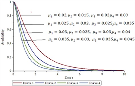
The Table 2 and Fig. 2 presents four different cases of system performance through system availability measures for different four cases of illustrations when the set of failure and repair values when the parameter of subsystems are highlighted as: $μ_{1} = 0.02,$ $μ_{2} = 0.015,$ $μ_{3} = 0.02$ , $μ_{4} =$ 0.03, $φ_{i} (x) =$ 1, $i =$ 1, 2, 3, $μ_{0} (x) =$ 2.7183, $n =$ 100, $k =$ 30, $μ_{1} =$ 0.025, $μ_{2} =$ 0.02, $μ_{3} =$ 0.025, $μ_{4} =$ 0.035, $φ_{i} (x) =$ 1, $i =$ 1, 2, 3, $μ_{0} (x) =$ 2.7183, $n =$ 100, $k =$ 30, $μ_{1} =$ 0.03, $μ_{2} =$ 0.025, $μ_{3} =$ 0.03, $μ_{4} =$ 0.04, $φ_{i} (x) =$ 1, $i =$ 1, 2, 3, $μ_{0} (x) =$ 2.7183, $n =$ 100, $k =$ 30 and $μ_{1} =$ 0.035, $μ_{2} =$ 0.03, $μ_{3} =$ 0.035, $μ_{4} =$ 0.045, $φ_{i} (x) =$ 1, $i =$ 1, 2, 3, $μ_{0} (x) =$ 2.7183, $n =$ 100, $k =$ 30 respectively. From Fig. 2 concludes the first case of illustration is the more acceptable and the fourth case is least beneficial for system operation.

2.2. Reliability Analysis.

Reliability is a metric of system performance of a non-repairable system. Therefor assuming all repair equal to zero in Eq. (66), and taking inverse Laplace transform of Eq. (66) keeping fix values of $k =$ 30, $n =$ 100, one may have expressions: $R_{1}$ , $R_{2}$ , $R_{3}$ and $R_{4}$ for the system reliability for given values of failure rates: Lets fix the failure and repair in Eq. (66) as; (i) $μ_{1} =$ 0.02, $μ_{2} = 0.015,$ $μ_{3} = 0.02$ , $μ_{4} = 0.03$ , (ii) $μ_{1} =$ 0.025, $μ_{2} = 0.020,$ $μ_{3} =$ 0.025, $μ_{4} = 0.035$ , (iii) $μ_{1} =$ 0.030, $μ_{2} = 0.025,$ $μ_{3} = 0.03$ , $μ_{4} =$ 0.040, (iv) $μ_{1} =$ 0.035, $μ_{2} = 0.030,$ $μ_{3} = 0.035$ , $μ_{4} =$ 0.045 in Eq. (66), one can get an expressions of the reliability of the system as:

68

R 1 = 3.846153846 e^{- 0.7350000000 t} - 3.093391608 e^{- 0.9300000000 t} + 0.0454545454545 e^{- 0.05000000000 t} + 0.03409090909 e^{- 0.6000000000 t} + 0.1676923077 e^{- 0.1500000000 t},

R 2 = - 3.496270562 e^{- 1.215000000 t} + 0.04819277108 e^{- 0.8000000000 t} + 0.1494685990 e^{- 0.1800000000 t} + 0.04329004329 e^{- 0.06000000000 t} + 4.255319149 e^{- 0.19800000000 t},

R 3 = 0.06250000000 e^{- 1 . t} + 4.545454545 e^{- 1.225000000 t} - 3.788827316 e^{- 1.500000000 t} + 0.1389147287 e^{- 0.2100000000 t} + 0.04195804196 e^{- 0.07000000000 t},

R 4 = - 3.496270562 e^{- 1.215000000 t} + 0.04819277108 e^{- 0.8000000000 t} + 0.1494685990 e^{- 0.1800000000 t} + 0.04329004329 e^{- 0.06000000000 t} + 4.255319149 e^{- 0.9800000000 t} .

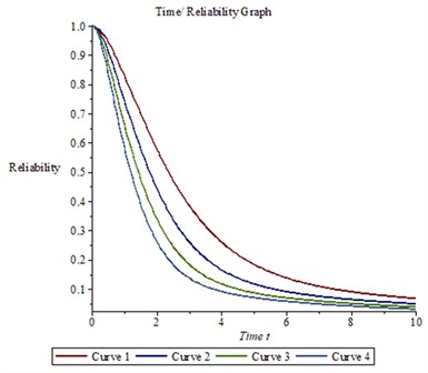
The Table 3 and Fig. 3 presents four different cases of system performance through system reliability measures for different four cases of illustrations when the set of failure and repair values when the parameter of subsystems are highlighted as: $μ_{1} =$ 0.02, $μ_{2} =$ 0.015, $μ_{3} =$ 0.02, $μ_{4} =$ 0.03, $φ_{i} (x) =$ 0, $i =$ 1, 2, 3, $μ_{0} (x) =$ 0, $μ_{1} =$ 0.025, $μ_{2} =$ 0.02, $μ_{3} =$ 0.025, $μ_{4} =$ 0.035, $φ_{i} (x) =$ 0, $i =$ 1, 2, 3, $μ_{0} (x) =$ 0, $μ_{1} =$ 0.03, $μ_{2} =$ 0.025, $μ_{3} = 0.03$ , $μ_{4} =$ 0.04, $φ_{i} (x) =$ 0, $i =$ 1, 2, 3, $μ_{0} (x) = 0$ and $μ_{1} = 0.035,$ $μ_{2} = 0.03,$ $μ_{3} = 0.035$ , $μ_{4} =$ 0.045, $φ_{i} (x) =$ 0, $i =$ 1, 2, 3, $μ_{0} (x) = 0$ respectively. From Fig. 3 concludes the first case of illustration is the more acceptable and the fourth case is least beneficial for system operation.

Table 3Variation of reliability regarding time

Time ( $t$ )	Reliability
Time ( $t$ )	Case R1	Case R2	Case R3	Case R4
0	1.000	1.000	1.000	1.000
1	0.830	0.747	0.665	0.587
2	0.578	0.444	0.340	0.262
3	0.385	0.261	0.184	0.138
4	0.260	0.166	0.117	0.091
5	0.184	0.117	0.086	0.070
6	0.137	0.908	0.096	0.057
7	0.109	0.075	0.058	0.048
8	0.090	0.064	0.050	0.041
9	0.077	0.055	0.043	0.035

Fig. 3Time reliability graph

2.3. Profit analysis/ cost analysis

For the same set of the parametric values that used in Eq. (66), one can get the expression for an expected profit of the system in interval $[0, t)$ : Taking the failure rates of the system as $μ_{1} =$ 0.02, $μ_{2} =$ 0.015, $μ_{3} =$ 0.02, $μ_{4} =$ 0.03 and repair $φ_{i} (x) =$ 1, $i =$ 1, 2, 3, ${\bar{S}}_{μ_{0}} (s) = \frac{\exp [x^{θ} + {\log φ (x)}^{θ}]^{1 / θ}}{s + \exp [x^{θ} + {\log φ (x)}^{θ}]^{1 / θ}}$ , $x =$ 1, $θ =$ 1, $φ_{i} (x) =$ 1, $i =$ 1, 2, 3 and assuming the repair facility is always available. Knowing the revenue generation ( $K_{1}$ ) and service cost ( $K_{2}$ ) per unit time in the interval $[0, t)$ , we can compute the predicted expected profit with the given formula:

E_{p} (t) = K_{1} \int_{0}^{t} P_{u p} (t) d t - K_{2} t .

Hence:

69

E_{p} (t) = K_{1} (- {0.004510942 e}^{- 2.801194514 t} + {0.0596403 e}^{- 2.270844668 t}

- {0.00442774 e}^{- 1.0647340 t} {- 0.00117862 e}^{- 1.60000 t} + 4.9325) - K_{2} (t) .

Setting $K_{1} =$ 1 and $K_{2} =$ 0.6, 0.4, 0.2 and 0.1 respectively and varying $t =$ 0, 1, 2, 3, 4, 5, 6, 7, 8, 9…one gets table 3. The corresponding figure 3 represents the variation of profit respect time $t$ .

Table 4Expected profit in 0,t: t= 0, 1, 2, 3,… ,9

Time $t$	$K_{1} =$ 1, $K_{2} =$ 0.6	$K_{1} =$ 1, $K_{2} =$ 0.5	$K_{1} =$ 1, $K_{2} =$ 0.4	$K_{1} =$ 1, $K_{2} =$ 0.2	$K_{1} =$ 1, $K_{2} =$ 0.1
0	0.0	0.0	0.0	0.0	0.0
1	0.350	0.451	0.550	0.750	0.851
2	0.540	0.741	0.940	1.340	1.541
3	0.574	0.875	1.1749	1.774	2.075
4	0.483	0.883	1.283	2.083	2.483
5	0.290	0.790	1.290	2.290	2.790
6	0.016	0.616	1.216	2.416	2.016
7	0.0	0.378	1.077	2.477	3.177
8	0.0	0.087	0.887	2.487	3.287
9	0.0	0.0	0.655	2.455	3.355

Fig. 4Expected profit graph for copula repair

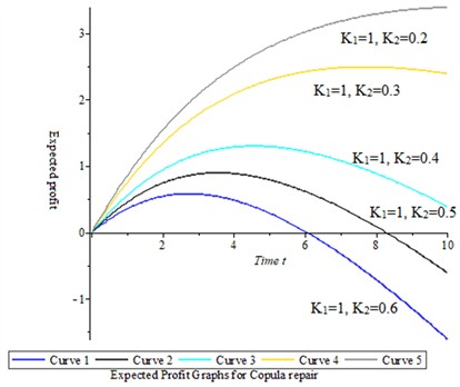
The Table 4 and Fig. 4 presents five different cases of expected profit for system through system availability measures for different five cases of illustrations when the set of failure and repair values when the parameter of subsystems are highlighted as: $μ_{1} = 0.02,$ $μ_{2} = 0.015,$ $μ_{3} = 0.02$ , $μ_{4} =$ 0.03, $φ_{i} (x) =$ 1, $i =$ 1, 2, 3, $μ_{0} (x) =$ 2.7183, $n =$ 100 and $k =$ 30 (30-out-of-100:G). The curve 1, curve 2, curve 3, curve 4 and curve 5 shows the expected profit variation for the values of $K_{1} =$ 1 and $K_{2} =$ 0.6, 0.5, 0.4, 0.3, 0.2, 0.1 respectively. From Fig. 4 the expected profit in time interval $[0, t)$ decreases when the service cost per unit increases.

3. MTTF analysis

Meaning Time to Failure, or MTTF, is a crucial reliability indicator that calculates how long an item that cannot be repaired typically lasts before failing. Because it enables businesses to anticipate component failure and preemptively plan for replacement, this statistic is essential for asset management. Maintenance lineups can create efficient preventative maintenance programs that reduce expensive repairs and improve overall system reliability by realizing MTTF. A key component of strategic maintenance planning, MTTF, is especially pertinent for possessions and equipment that cannot or should not be fixed.

Conserving to the above treating all repairs rates $φ_{i} (x) =$ 0, $i =$ 1, 2, 3, $μ_{0} (x) = 0$ in ${\bar{P}}_{u p} (s)$ and $M T T F = \lim_{s \to 0} {\bar{P}}_{u p} (s)$ treating repairs to zero in Eq. (66). i.e.:

70

M T T F = \frac{1}{(μ_{1} + n μ_{2} + {2 μ}_{3} + {4 μ}_{4})} (1 + \frac{n μ_{2}}{(n - 1) μ_{2}} + \frac{n (n - 1) {μ_{2}}^{2}}{(n - k) μ_{2}} + \frac{n (n - 1) (n - k) {μ_{2}}^{3}}{(n - k - 1) μ_{2}} + \frac{{2 μ}_{3} (1 + {4 μ}_{4} + {12 μ}_{1}^{2})}{μ_{4} + μ_{3}}) .

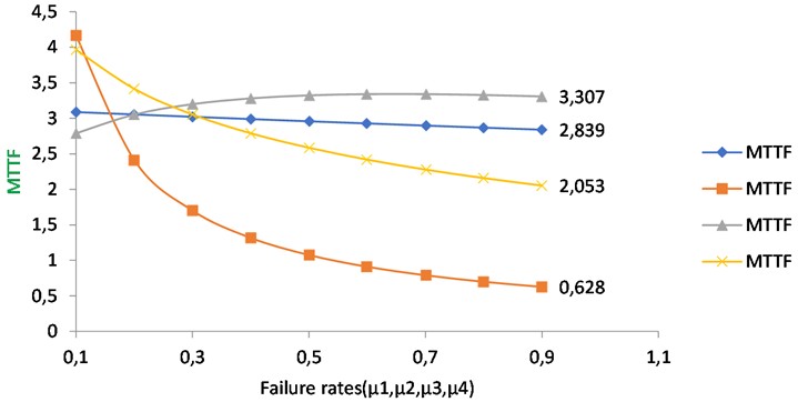
We may obtain the values of the MTTF corresponding to the failure rate $μ_{1}$ by fixing $μ_{2} =$ 0.015, $μ_{3} =$ 0.02, and $μ_{4} =$ 0.03 and altering $μ_{1}$ as follows: 0.1, 0.2, 0.3, 0.4, 0.5, 0.6, 0.7, 0.8, and 0.9 in Eq. (70). Table 5 column 2 displays the MTTF change regarding failure1.

By adjusting $μ_{1} =$ 0.02, $μ_{3} =$ 0.02, and $μ_{4} =$ 0.03 and modifying $μ_{3}$ as follows: 0.1, 0.2, 0.3, 0.4, 0.5, 0.6, 0.7, 0.8, and 0.9 in Eq. (70), one may determine the MTTF values that correlate to the failure rate $μ_{3}$ . Table 5 column 4 displays the MTTF fluctuation in relation to failure rate $μ_{3}$ .

Restoring, $μ_{1} =$ 0.02, $μ_{2} =$ 0.015, and, $μ_{3} =$ 0.02, and altering $μ_{4}$ as; 0.1, 0.2, 0.3, 0.4, 0.5, 0.6, 0.7, 0.8, 0.9 in Eq. (70) we can obtain the values of MTTF corresponding to the failure rate $μ_{4}$ . Column 5 of table 5 shows the difference of MTTF with respect to the failure $μ_{4}$ .

Table 5Variation of MTTF with failure rates.

Failure rates	MTTF ( $μ_{1})$	MTTF $(μ_{2})$	MTTF ${(μ}_{3})$	MTTF ${(μ}_{4})$
0.1	3.0863	4.166	2.790	3.967
0.2	3.0531	2.411	3.053	3.415
0.3	3.020	1.701	3.199	3.053
0.4	2.988	1.317	3.280	2.789
0.5	2.957	1.076	3.322	2.585
0.6	2.927	0.911	3.339	2.418
0.7	2.897	0.791	3.339	2.278
0.8	2.868	0.700	3.327	2.158
0.9	2.839	0.628	3.307	2.053

Fig. 5variation of MTTF with failure rates

4. Sensitivity analysis

Sensitivity analysis is the study of how various sources of input uncertainty might be assigned to the uncertainty in a mathematical model or system output. This entails calculating sensitivity indices, which measure how much an input or set of inputs affects the result. Ambiguity and sensitivity analysis should ideally be conducted together. Vagueness analysis is a similar activity that focuses more on the enumeration and spread of uncertainty.

Mathematically, sensitivity with respect to a particular parameter can be obtained by partial derivative of function with respect to the given variable. Since MTTF is a function of failure rates. The variation of partial derivative with respect to the failure rates while fixing the other failure rates gives the sensitivity analysis of the MTTF regarding failure rates.

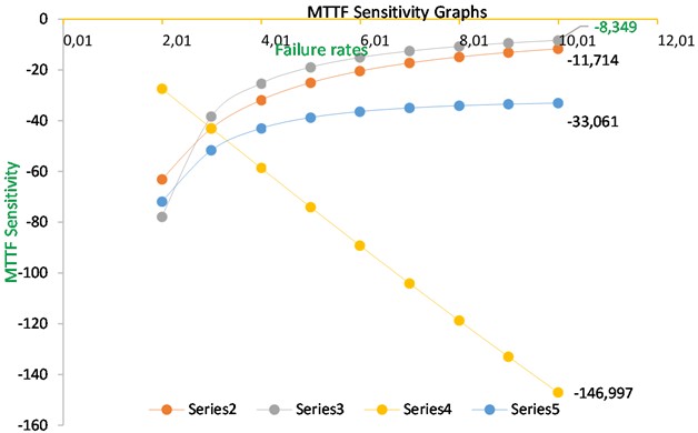
Sensitivity analysis for change in MTTF resulting from changes in the system parameters, i.e. system failure rates $μ_{1}$ , $μ_{2}$ , $μ_{3}$ and $μ_{4}$ . Differentiating MTTF Eq. (70) with respect to failure rates $μ_{1}$ , $μ_{2}$ , $μ_{3}$ and $μ_{4}$ ( $\partial (M T T F) / \partial μ_{j}$ , $j =$ 1, 2, 3, 4), while holding other failure rates constant, yields the values shown in Table 6.

Table 6Sensitivity of MTTF with failure rates

Failure rate	$\frac{\partial (M T T F)}{\partial μ_{1}}$	$\frac{\partial (M T T F)}{\partial μ_{2}}$	$\frac{\partial (M T T F)}{\partial μ_{3}}$	$\frac{\partial (M T T F)}{\partial μ_{4}}$
0.01	–63.144	–77.893	–27.441	–71.908
0.02	–43.039	–38.356	–43.039	–51.637
0.03	–31.908	–25.373	–58.617	–43.039
0.04	–25.048	–18.944	–74.028	–38.763
0.05	–20.487	–15.112	–89.201	–36.400
0.06	–17.278	–12.568	–104.098	–34.988
0.07	–14.918	–10.756	–118.700	–34.091
0.08	–13.122	–9.401	–133.000	–33.487
0.09	–11.714	–8.349	–146.997	–33.061

Fig. 6MTTF Sensitivity variation respect to failure rates

5. Result discussion and interpretation of the results

In the present manuscript, the authors computed the performance of system reliability metrics of a complex system comprised of the four subsystems in series configuration. Fig. 1(a) and 1(b) is the system configuration and state transition diagram of mathematical model which presents the system architecture and the possible transition in the states. Table 2 and the corresponding Fig. 2 show the system performance of repairable systems through multi repair approach. However, it was evidently observed that the system performance decreases when the failure rates values were enhanced. The best performance was seen for case 1 of computations and low performance for case 4 when failure rates were comparably high. The reliability metric can be predicted as the performance of a non-repairable system. The reliability variation with time is highlighted in Table 3 and Fig. 3; a clear decrease in the reliability function is observed for all four cases, exceeding the decrease in availability. The same observations were found as high failure rates of subsystems low reliability. Table 4 and the attached figure 4 show the system profit analysis corresponding to allocated failure and repair parameters of the repairable system. The fundamental fact found true when service cost per unit item interval $[0, t)$ increases the net profit for running, the system decreases and when service cost per unit item decreases, the net profit increases. Table 5 presents the MTTF metric for the system, which predicts the average time of failure respect to failure rates. By Fig. 5 we conclude that the MTTF variation trend is decreased at a high rate for the failure rate of subsystem 2 with failure rate $μ_{2}$ which works for the k-out-of-n: G scheme. MTTF for failure rate of subsystem 3 with failure rate $μ_{3}$ is increasing trend but MTTF for subsystem 4i.e., $μ_{4}$ is decreasing trend. The trend of MTTF for subsystem 1 is almost fixed. Table 6 and Fig. 6 of the analysis presents the sensitivity analysis of mean time to failure MTTF corresponding to varying the failure rates of subsystems. By Fig. 6, it has been concentrated that the sensitivity decreases for the subsystem 3 but for subsystem 2, subsystem 3 and subsystem 4 is not seriously affected. In applications where the system's value is limited, this approach is especially helpful for design engineers who prioritize reliability since it makes it possible to choose components that are both efficient and of good quality. The application of comparable integrated reliability models in reliability engineering contexts can be improved by building them with redundancy by utilizing modern heuristic techniques.

In the current paper, a system comprising four subsystems is analyzed. The third subsystem consists of two identical load balancers, which may be extended to non-identical load balancers or number of load balancers, can be increased and impact of system performance could be analyses. Also, in the subsystem four identical units’ subsystem have assumed it can be extended to extra units and non-identical also and the results can be compared for various reliability metrics.

References

H. W. Block, R. E. Barlow, and F. Proshan, “Statistical theory of reliability and life testing: probability models,” Journal of the American Statistical Association, Vol. 72, No. 357, p. 227, Mar. 1977, https://doi.org/10.2307/2286944

Publisher
H. Joe, Multivariate Models and Dependent Concepts. London: Champman & Hall, 1997.

Publisher
D. R. Cox, “The analysis of non-Markovian stochastic processes by the inclusion of supplementary variables,” Mathematical Proceedings of the Cambridge Philosophical Society, Vol. 51, No. 3, pp. 433–441, Oct. 2008, https://doi.org/10.1017/s0305004100030437

Publisher
R. B. Nelson, An Introduction to Copulas. New York: Springer, 2006.

Search CrossRef
A. Kumar and S. Malik, “Reliability modelling of a computer system with priority to H/W repair over replacement of H/W and up-gradation of S/W subject to MOT and MRT,” Jordan Journal of Mechanical and Industrial Engineering, JJMIE, Vol. 8, No. 4, pp. 233–241, 2014.

Search CrossRef
Chiwa Musa Dalah and V. V. Singh, “Study of reliability measures of a two units standby system under the concept of switch failure using copula distribution,” American Journal of Computational and Applied Mathematics, Vol. 4, No. 4, pp. 118–129, 2014, https://doi.org/10.5923/j.ajcam.20140404.02

Publisher
V. V. Singh and J. Gulati, “Availability and cost analysis of a standby complex system with different types of failure under waiting repair discipline using Gumbel-Hougaard family copula distribution,” in International Conference on Issues and Challenges in Intelligent Computing Techniques (ICICT), pp. 180–186, Feb. 2014, https://doi.org/10.1109/icicict.2014.6781275

Publisher
I. Yusuf and B. Yusuf, “Reliability comparison between redundant repairable network flow systems,” SOP Transactions on Applied Mathematics, Vol. 1, No. 1, pp. 42–59, Mar. 2014, https://doi.org/10.15764/am.2014.01005

Publisher
A. Mishra, “Availability of k-out-of-n: F Secondary subsystem with general repair time distribution,” International Journal of Engineering, Vol. 26, No. 7(A), pp. 74–752, Jul. 2013, https://doi.org/10.5829/idosi.ije.2013.26.07a.09

Publisher
D. K. Rawal, S. K. Sahani, V. V. Singh, and A. Jibril, “Reliability assessment of multi-computer system consisting n clients and the k-out-of-n: G operation scheme with copula repair policy,” Life Cycle Reliability and Safety Engineering, Vol. 11, No. 2, pp. 163–175, May 2022, https://doi.org/10.1007/s41872-022-00192-5

Publisher
K. G. Ramamurthy, “Reliability function of consecutive k-out-of-n systems for the general case,” Sankhya B: Indian journal of Statistics, Vol. 59, pp. 396–420, 1997.

Search CrossRef
Xiaolin Liang, Yinfeng Xiong, and Zehui Li, “Exact Reliability formula for consecutive k-out-of-n repairable systems,” IEEE Transactions on Reliability, Vol. 59, No. 2, pp. 313–318, Jun. 2010, https://doi.org/10.1109/tr.2010.2046790

Publisher
V. V. Singh and D. K. Rawal, “Availability analysis of a system having two units in a series configuration with the controller and human failure under different repair policies,” International Journal of Scientific and Engineering Research, Vol. 2, No. 10, pp. 1–9, 2011.

Search CrossRef
K. Vijaykumar and R. P. Kumudinidevi, “A new method for optimal location of FACTS controllers using Genetic Algorithm,” Journal of Theoretical and Applied Information Technology, Vol. 3, No. 4, pp. 1–6, 2007.

Search CrossRef
Y. Ibrahim, B. Yusuf, M. Babagana, B. Sani, and M. A. Lawan, “Some reliability characteristics of a linear consecutive 2-out-of-4 system connected to 2-out-of-4 supporting device for operation,” International Journal of Engineering and Technology, Vol. 7, No. 1, pp. 135–139, Feb. 2018, https://doi.org/10.14419/ijet.v7i1.8037

Publisher
P. K. Poonia, “Performance assessment and sensitivity analysis of a computer lab network through copula repair with catastrophic failure,” Journal of Reliability and Statistical Studies, Vol. 15, No. 1, pp. 105–128, Mar. 2022, https://doi.org/10.13052/jrss0974-8024.1515

Publisher
V. Singh and P. K. Poonia, “Stochastic analysis of k-out-of-n: G type of repairable system in combination of subsystems with controllers and multi repair approach,” Journal of Optimization in Industrial Engineering, Vol. 15, No. 1, pp. 121–130, Jun. 2022, https://doi.org/10.22094/joie.2021.1906935.1780

Publisher
D. Raghav, Shakeeludeen, S. K. Sahani, and V. V. Singh, “Performance assessment of complex repairable system with k-out-of-n: G operational scheme and copula repair approach,” Journal of Industrial Engineering International, Vol. 18, No. 3, pp. 35–49, 2023, https://doi.org/10.30495/jiei.2023.1953669.1210

Publisher
A. Kumar, R. Garg, and M. S. Barak, “Performance of computer system with three types of failure using weibull distribution subject to hardware repair and software up-gradation,” International Journal of System Assurance Engineering and Management, Vol. 14, No. S1, pp. 483–491, Mar. 2023, https://doi.org/10.1007/s13198-023-01879-3

Publisher
H. I. Ayagi, V. V. Singh, and Z. Wan, “Stochastic assessment of k operational state system with k-out-of-n:G working scheme with employing copula repair approach,” International Journal of Reliability, Quality and Safety Engineering, Vol. 30, No. 2, Apr. 2023, https://doi.org/10.1142/s0218539323500043

Publisher
M. Saini and A. Kumar, “Sensitivity analysis and RAMD investigation of ghee producing unit of milk plant,” Jordan Journal of Mathematics and Statistics, Vol. 17, No. 4, pp. 483–491, 2024.

Search CrossRef
V. V. Singh, J. Paliwal, and M. Yadav, “Probabilistic assessment of n clients network system covering four subsystems and non-identical load balancers,” Life Cycle Reliability and Safety Engineering, Feb. 2025, https://doi.org/10.1007/s41872-024-00292-4

Publisher
A. T. Alhasani, A. Hussein, A. S. Alhumaima, M. E. El-Sayed, and M. E.-E. Marwa, “A comparative analysis of methods for detecting and diagnosing breast cancer based on data mining,” Journal of Artificial Intelligence and Metaheuristics, Vol. 4, No. 2, pp. 08–17, Jan. 2023, https://doi.org/10.54216/jaim.040201

Publisher
M. Mahmoud, “A review on waste management techniques for sustainable energy production,” Metaheuristic Optimization Review, Vol. 3, No. 2, pp. 47–58, Jan. 2025, https://doi.org/10.54216/mor.030205

Publisher
A. Hobiny, I. Abbas, and M. Marin, “The influences of the hyperbolic two-temperatures theory on waves propagation in a semiconductor material containing spherical cavity,” Mathematics, Vol. 10, No. 1, p. 121, Jan. 2022, https://doi.org/10.3390/math10010121

Publisher
E.-S. M. El-Kenawy, N. Khodadadi, S. Mirjalili, A. A. Abdelhamid, M. M. Eid, and A. Ibrahim, “Greylag goose optimization: nature-inspired optimization algorithm,” Expert Systems with Applications, Vol. 238, No. Part E, p. 122147, Mar. 2024, https://doi.org/10.1016/j.eswa.2023.122147

Publisher
N. Khodadadi, L. Abualigah, E.-S. M. El-Kenawy, V. Snasel, and S. Mirjalili, “An archive-based multi-objective arithmetic optimization algorithm for solving industrial engineering problems,” IEEE Access, Vol. 10, pp. 106673–106698, Jan. 2022, https://doi.org/10.1109/access.2022.3212081

Publisher

About this article

Received

13 March 2025

Accepted

17 July 2025

Published

16 August 2025

DOI

https://doi.org/10.21595/mme.2025.24893

Keywords

k-out-of-n: G system configuration

system availability measure

system reliability measure

MTSF

sensitivity analysis

profit analysis

Gumbel-Hougaard family copula distribution

Acknowledgements

The authors have not disclosed any funding.

Data Availability

The datasets generated during and/or analyzed during the current study are available from the corresponding author on reasonable request.

Author Contributions

Shailly Sharama have prepared the article under the supervision of Prof. V. V. Singh and Dr. Priyavada. Prof. V. V. Singh rewrites the final draft of this paper.

Conflict of interest

The authors declare that they have no conflict of interest.

This is an open access article distributed under the Creative Commons Attribution License, which permits unrestricted use, distribution, and reproduction in any medium, provided the original work is properly cited.

S. Sharma, V. V. Singh, P. Parihar, and P. L. Neupane, “Performance assessment of network system network comprising four subsystems via multi failure and multi repair methodology,” Mathematical Models in Engineering, Vol. 11, No. 3, –18, Aug. 2025, https://doi.org/10.21595/mme.2025.24893

Copy Extrica

Copied to clipboard!

TY  - JOUR
DO  - 10.21595/mme.2025.24893
UR  - https://doi.org/10.21595/mme.2025.24893
TI  - Performance assessment of network system network comprising four subsystems via multi failure and multi repair methodology
T2  - Mathematical Models in Engineering
AU  - Sharma, Shailly
AU  - Singh, V. V.
AU  - Parihar, Priyavada
AU  - Neupane, Padam Lal
PY  - 2025
DA  - 2025/08/16
PB  - Extrica
VL  - 11
IS  - 3
SN  - 2351-5279
SN  - 2424-4627
ER  - 

Copy Ris

Copied to clipboard!

 @article{Sharma_2025, title={Performance assessment of network system network comprising four subsystems via multi failure and multi repair methodology}, ISSN={2424-4627}, url={https://doi.org/10.21595/mme.2025.24893}, DOI={10.21595/mme.2025.24893}, journal={Mathematical Models in Engineering}, publisher={JVE International Ltd.}, author={Sharma, Shailly and Singh, V. V. and Parihar, Priyavada and Neupane, Padam Lal}, year={2025}, month=aug }

Copy Bibtex

Copied to clipboard!

[1]S. Sharma, V. V. Singh, P. Parihar, and P. L. Neupane, “Performance assessment of network system network comprising four subsystems via multi failure and multi repair methodology,” Mathematical Models in Engineering, Aug. 2025, doi: 10.21595/mme.2025.24893.

Copy IEEE

Copied to clipboard!

Sharma, Shailly, V. V. Singh, Priyavada Parihar, and Padam Lal Neupane. “Performance Assessment of Network System Network Comprising Four Subsystems via Multi Failure and Multi Repair Methodology.” Mathematical Models in Engineering, August 16, 2025. https://doi.org/10.21595/mme.2025.24893.

Copy Chicago

Copied to clipboard!

Performance assessment of network system network comprising four subsystems via multi failure and multi repair methodology

Abstract

1. Introduction

1.1. State description of the model

1.2. Mathematical modeling of the model

2. Analysis and discussion of results

2.1. Availability analysis

2.2. Reliability Analysis.

2.3. Profit analysis/ cost analysis

3. MTTF analysis

4. Sensitivity analysis

5. Result discussion and interpretation of the results

References

About this article

Related Articles