Abstract
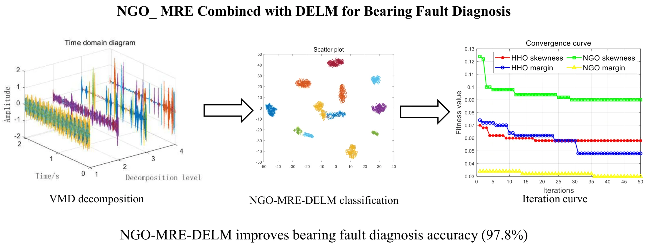
To improve the effectiveness of Multiscale Range Entropy (MRE) in extracting features from rolling bearing faults, this paper proposes a novel bearing fault diagnosis method that combines the Northern Goshawk Optimization (NGO) algorithm, MRE, and a Deep Extreme Learning Machine (DELM). First, the raw vibration signal is decomposed using Variational Mode Decomposition (VMD) to obtain its Intrinsic Mode Functions (IMFs). Second, the NGO algorithm is employed to optimize the MRE parameters, using the minimum crest factor as the objective function. Then, using these optimized parameters, MRE is applied to extract fault features. The resulting feature set undergoes dimensionality reduction to create the final sample set. Finally, an NGO-optimized DELM is used for fault classification. The experimental results demonstrate that this method effectively extracts the characteristic signals of rolling bearing faults through robust parameter optimization, thereby improving the accuracy of fault diagnosis.
Highlights
- Developed an NGO-MRE-DELM framework for bearing fault diagnosis, integrating VMD decomposition, parameter optimization, and deep learning to improve accuracy.
- Demonstrated that optimizing MRE with the minimum margin factor significantly enhances feature extraction, achieving 97.8% fault recognition accuracy.
- The NGO algorithm improved both speed and reliability of parameter optimization, outperforming traditional methods by avoiding premature convergence and reducing computation time.
1. Introduction
Rolling bearings are indispensable components in rotating machinery. Their failure can cause significant machinery malfunction and severe losses. Therefore, accurate and timely fault identification – locating the fault and determining its type – is crucial [1].
Extracting informative features from vibration signals is a cornerstone of fault diagnosis methodologies. The integration of feature extraction techniques with domain expertise and signal processing methods continues to deepen [2].
Recent advances in nonlinear theory, particularly entropy-based feature extraction methods, have found widespread application in this field [3]. Concurrently, time-domain vibration analysis remains vital for rotating machinery fault diagnosis. For instance, Pająk [4] investigated the use of time-domain features like skewness and kurtosis for bearing fault detection, demonstrating their potential in complex machinery systems. Analyzing signals across multiple time scales enhances the extraction of fault characteristics, making multi-scale entropy (MSE) a popular tool [5]. Examples include Multi-scale Fuzzy Entropy (MFE) [6], Multi-scale Permutation Entropy (MPE) [7], and Multi-scale Sample Entropy (MSE) [8].
However, a key challenge in engineering practice is parameter selection for fault diagnosis, which often relies heavily on empirical knowledge and lacks adaptability [9]. Multi-scale entropy methods face similar issues; for example, selecting appropriate scale factors and time series lengths for MPE remains non-trivial [10]. Consequently, selecting optimal parameters is critical for effective feature extraction. Furthermore, choosing a suitable objective function as the optimization criterion is essential to ensure the scientific validity and reliability of the selected parameters.
Previous research highlights different approaches: Wang Haiming et al. [11] employed a Particle Swarm Optimization (PSO) algorithm to select MPE parameters for rolling bearing fault identification, using the squared skewness function as the objective function. Zhang Min [12], in a method based on adaptive Maximum Correlated Kurtosis Deconvolution (MCKD) and VMD, determined optimized parameters using maximum permutation entropy and maximum kurtosis, overcoming the limitations of manual parameter selection.
Among potential objective function candidates, the crest factor – a dimensionless parameter representing the ratio of signal peak to root mean square (RMS) amplitude – demonstrates superior sensitivity and stability for fault characteristic signals compared to other indicators. It effectively reflects fault-related information. Therefore, this paper selects the minimization of the crest factor as the objective function to optimize MRE parameters (embedding dimension ** and tolerance **), aiming to obtain the most suitable values.
Selecting an appropriate optimization algorithm is equally important. Traditional algorithms like Genetic Algorithms (GA) [13] and PSO [14] often suffer from long optimization times and slow convergence. The Northern Goshawk Optimization (NGO) algorithm, a novel intelligent optimization technique, offers faster convergence [15]. Comparative studies by Mohammad et al. [16] found that NGO outperforms various traditional algorithms in solving optimization problems, achieving better results more efficiently with less computational time. Consequently, the NGO algorithm is adopted as the primary parameter optimization method in this work.
Finally, utilizing the optimized MRE parameters to extract features and subsequently employing these features for fault recognition is key to bearing fault diagnosis. Various intelligent classifiers have been applied, such as Grey Wolf Optimized Support Vector Machines (GWO-SVM) [17] and Weighted Domain Adaptive Convolutional Neural Networks (WDA-CNN) [18]. Deep learning models are also prevalent. For example, Song Jiangtao et al. [19] combined a decomposed NGO-VMD residual term with Long Short-Term Memory (LSTM) for prediction, while Wang Yuhong et al. [20] used an improved Whale Optimization Algorithm (WOA) to optimize a Kernel Extreme Learning Machine (KELM) model, enhancing accuracy and generalization.
The Extreme Learning Machine (ELM), based on single hidden-layer feedforward neural networks with randomly assigned input weights and biases, offers high accuracy and fast training [21, 22]. However, its classification performance can degrade under varying working conditions or noisy environments. Integrating ELM with deep learning architectures addresses these limitations, improving robustness and stability while mitigating tedious training processes [23]. Therefore, this paper employs a Deep Extreme Learning Machine (DELM) and utilizes the NGO algorithm to optimize its parameters, accelerating target search and convergence.
Leveraging the aforementioned advantages, this study proposes a comprehensive bearing fault diagnosis method: 1) VMD decomposes bearing vibration data into Intrinsic Mode Functions (IMFs); 2) Using the minimum crest factor as the objective function, the NGO algorithm optimizes MRE parameters; 3) Optimized MRE extracts multi-scale fault features; 4) Isometric Mapping (ISOMAP) reduces feature dimensionality; 5) NGO-optimized DELM performs fault classification. Experimental results validate the speed and accuracy of this approach.
2. Theoretical foundation
2.1. Multi scale range entropy
RE is a nonlinear method proposed by Amir in 2018, which can more accurately and effectively measure complex nonlinear time series. However, due to the fact that rolling bearing fault signals are generally distributed on multiple scales, MRE is used to obtain fault information at multiple scales [24]. The specific formula is as follows:
Reconstruct the phase space and give a time series of length , is . Select data points and reconstruct the sequence in the original order to obtain , as shown in the calculation:
where, and represent the embedding dimension and delay time, respectively. When , the original data is split into a new sequence to obtain the reconstructed sequence.
Using rescaled range analysis, calculate the distance between and other subsequences . The formula is:
Compare the difference between each and similar capacity , and calculate that satisfies the sum of , as follows:
where , is the Heaviside function, calculated as follows:
Add all A and take the mean to obtain the expression for B:
Repeat the above steps to obtain from , and then calculate RE using the following formula:
Coarse grained using the following formula:
where, is the scaling factor, is the coarse-grained time series, and is the rounding function. When , is the original time series.
Calculate the coarse-grained time series for each RE, and the MRE is obtained from the following formula:
2.2. NGO optimization algorithm
NGO is a new optimization algorithm proposed by Mohammad et al. [16] in 2021, and its mathematical model mainly consists of the following three parts:
1) Initialize the population. Randomly distribute the population in the search space, and the population matrix is:
where, represents the position of the northern eagle, represents the population size, represents the dimension for solving the problem, and represents the position of the dimension of the northern eagle.
The objective function value is expressed as a vector:
where, is the objective function vector of the population, and is the objective function value of the northern eagle.
2) Phase 1: Search and recognition phase. The northern eagle randomly selects a prey in the search space and conducts a global search to obtain the optimal region. Its mathematical model is as follows:
, represents the prey position of the northern eagle, represents the prey position of the northern eagle in the dimension, and is a random integer of ; is the new position of the northern eagle, is the new position of the northern eagle, and is its corresponding fitness value; The parameters and are new random numbers updated during the search and iteration process, where the interval is a random number of [0, 1] and the value of is 1 or 2;
3) Phase 2: Chasing and Escaping. During the pursuit of prey by the Northern Goshawk, the prey attempts to escape, and the Northern Goshawk will chase at an extremely fast speed and ultimately capture the prey. Assuming that the hunting range of the Northern Goshawk is radius . This simulation method increases the local search ability of NGOs in the search space, and its mathematical model is:
where, represents the updated position of the northern eagle after update; is the current number of iterations, and is the maximum number of iterations; refers to the new position of the northern eagle in , and is the objective function value of the northern eagle updated by .
2.3. Deep extreme learning machine
Extreme Learning Machine (ELM) is a single hidden layer feedforward neural network applied to supervised learning problems. Given samples , and represent the number of features and categories, respectively [25]. Its model is as follows:
where, is the output weight of the hidden layer node, is the input weight of the hidden layer node, is the threshold of the hidden layer node, and is the activation function. This article uses the sigmoid function.
The matrix expression of ELM:
By using the least squares solution , make:
Among them, is the output matrix of the hidden layer, is the expected output matrix of the sample, and the formula for the output weight is:
Among them, is the generalized inverse matrix of .
Applying the autoencoder AE to ELM, its weight is converted to:
Stacking multiple extreme learning machine autoencoders ELM-AE to form a DELM, the weights and biases of each ELM-AE random input will affect the final training results. In subsequent experiments, the Northern Eagle Optimization Algorithm will be introduced to optimize the parameters of the DELM.
3. Experimental data, steps, and parameter selection
3.1. Experimental data
The experimental data utilizes the publicly available Southeast University dataset, with bearing operating conditions categorized as 20-0 (20 Hz, 1200 rpm, unloaded, 0 V, 0 N/m) and 30-2 (30 Hz, 1800 rpm, loaded, 2 V, 7.32 N/m). The bearing conditions are divided into five types, namely: ball failure, inner ring failure, outer ring failure, inner and outer ring combination failure, and health status. The experimental setup is shown in the figure.
The data in its public dataset file has a total of 8 columns of vibration signals, and the 4th column of data in each type of dataset is selected for experiments in this paper. The summarized data types are 10 in total, and the selected data are labeled as follows in Table 1.
Fig. 1Southeast university bearing test stand
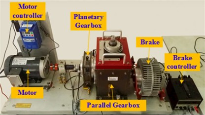
Table 1Marking of 10 bearing conditions
Bearing condition | Speed-load | label |
Ball failure | 20_0 | 1 |
30_2 | 2 | |
Inner and outer ring combination failure | 20_0 | 3 |
30_2 | 4 | |
Health status | 20_0 | 5 |
30_2 | 6 | |
Inner ring failure | 20_0 | 7 |
30_2 | 8 | |
Outer ring failure | 20_0 | 9 |
30_2 | 10 |
In Table 1, the bearing conditions selected are categorized into ball failure, inner race failure, outer race failure, outer race combined failure, and healthy state. The working environments are classified into two conditions: 1) rotational speed of 20 Hz (1200 rpm) with no load (0 V, 0 N/m), and 2) rotational speed of 30 Hz (1800 rpm) with a load of 2 V (7.32 N/m). These categories are presented across five rows. The reasons for these selections are as follows:
Representativeness: The chosen fault types cover common bearing failures, each with distinct vibration characteristics, allowing for a comprehensive evaluation of the diagnosis method.
Combination Failure: The inclusion of inner and outer ring combination failure is crucial as it presents more complex vibration patterns, making it harder to identify compared to single faults. This adds practical challenge to the experiment, as combination failures are common in real-world scenarios.
Health Status as Baseline: The health status serves as a reference for normal conditions, enabling comparison against fault states.
Data Diversity: These 5 rows offer sufficient fault variety while maintaining manageable data complexity for efficient analysis.
3.2. Experimental steps
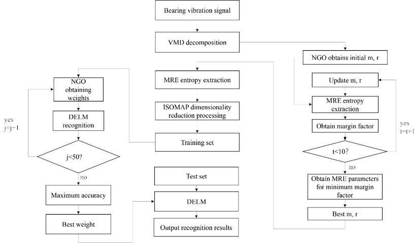
1) Using VMD to decompose the fault signal and obtain all IMF.
2) Select a portion of the intrinsic mode components and use the NGO optimization algorithm to optimize the and values of multi-scale range entropy based on the minimum margin factor.
3) Using the optimal sum value, calculate the range entropy of all data at different scales to obtain feature signals.
4) Using ISOMAP to reduce the dimensionality of feature signals and remove excess fault signals;
5) Using the DELM optimization algorithm of NGO to identify and classify the fault features after dimensionality reduction.
Fig. 2Experimental flow chart
3.3. Description of NGO algorithm parameter settings
Population Size: Set to 50 individuals. This setting aims to balance optimization stability and computational efficiency.
Maximum Number of Iterations: Set to 150 iterations, as the algorithm fully converges at this iteration count.
Search Space Boundaries: The search range for the optimization variable (DELM network weights) is limited to [–5, 5], based on the characteristics of the Sigmoid activation function.
Optimization Variable Dimension: The dimension is automatically determined by the DELM network structure.
Objective Function: The optimization objective is to minimize the classification error rate of the training set.
3.4. Parameter settings of Harris eagle optimization (HHO) algorithm
Table 2Parameter settings of Harris eagle optimization (HHO) algorithm
Population size | N | 50 | Be in line with ngo |
Max iterations | T | 150 | Be in line with ngo |
Primary energy | E0 | [–1, 1] random | standard setting |
Levi’s index | β | 1.5 | Heidari's original thesis |
Jump intensity | S | 0.01 | standard setting |
Dimensionality | D | 3720 | DELM network structure |
3.5. Fault diagnosis analysis
Select the bearing status data with a rotational speed of 20 Hz- no load (20-0) (including health status, ball faults, combined faults of inner and outer rings, inner ring faults and outer ring faults), process the original signal using VMD decomposition, select the default values of parameters, the number of modes 4 and the penalty factor 2000 [27], and obtain its time-domain graph and frequency domain graph as follows.
Fig. 3Time domain diagrams of VMD decomposition for different faults
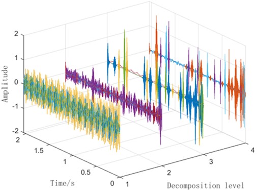
Fig. 4Spectrum diagram of VMD decomposition for different faults
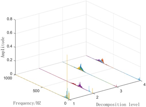
Fig. 3 reveals that the initial input signals overlap significantly prior to VMD decomposition, making it difficult to distinguish between their fault types. After performing VMD decomposition, partial separation of fault signal information becomes evident in IMF4. The accompanying time-domain plot and spectrogram further confirm the extraction of some time-frequency domain features. However, the figure also clearly shows that a substantial number of signals remain overlapping and difficult to identify, even after decomposition. This suggests that relying solely on VMD decomposition is insufficient for completely distinguishing between these five fault types under identical operating conditions.
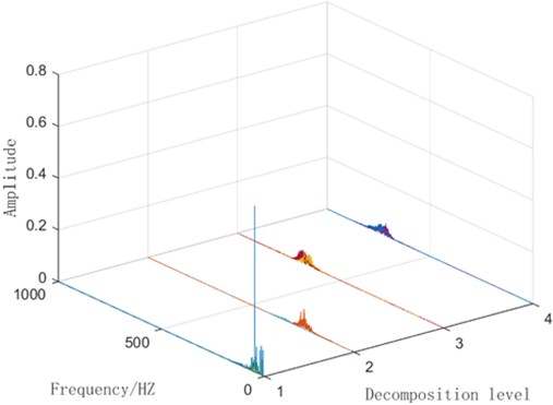
Moreover, analyzing the same type of fault (outer race fault) across different operating conditions further highlights this limitation. For example, comparing outer race fault signals under Condition 1 (20 Hz (1200 RPM) speed with 0 V (0 N/m) load) versus Condition 2 (30 Hz (1800 RPM) speed with 2 V (7.32 N/m) load) demonstrates that using VMD decomposition alone does not yield more effective fault information.
Specific results are shown in Figs. 5 to 6.
Therefore, after decomposing the VMD signal, further use the fault information obtained from MRE. However, due to the fact that the values of the embedding dimension and tolerance parameter in the MRE index will affect the final effectiveness of obtaining fault information, optimization algorithms are used to optimize the two parameters , of MRE before extracting fault information. Among them, there are 20 populations and 15 optimization iterations.
Fig. 5Time domain diagram after VMD decomposition of the same fault
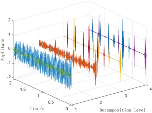
Fig. 6Spectrum diagram of VMD decomposition for the same fault
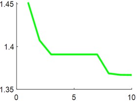
Select a single fault signal with a length of 1024, and use two optimization algorithms, NGO and HHO, to conduct experiments with the objective function of minimum skewness squared and minimum margin factor, where [1, 5] is an integer and [0.01, 1] is a random number. The iteration curve of the experiment is shown below.
From the comparison of Fig. 7(a, c), and (b, d), it can be seen that the convergence speed of the NGO algorithm under the same objective function is significantly faster than that of the HHO algorithm.
Select 100 fault signals with a length of 1024 as experimental data, and use MRE to extract fault characteristic signals based on the parameters obtained through optimization. The final fault characteristic signal dataset size is 100×128. Divide the feature signal dataset into training and testing sets, with sizes of 50×128, and conduct experiments.
Take the average entropy value of the original data and select the data from the first 50 sample points of one type of fault for analysis. Fig. 8 reveals two key findings regarding the performance of the HHO and NGO optimization algorithms. First, their performance on the profit rate indicators is strikingly similar, with the curves completely overlapping. This convergence likely arises from shared characteristics: both algorithms are based on swarm intelligence principles, optimize similar objectives (minimizing classification error, maximizing feature accuracy), and were tested under identical experimental conditions (population size, iterations) using the same dataset. The limited complexity of the dataset may have also restricted the diversity of potential solutions, causing both algorithms to converge on the same optimal point.
Fig. 7Iteration curve
a) HHO minimum skewness square
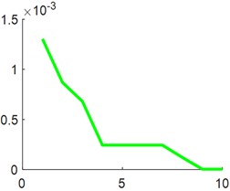
b) HHO minimum margin factor
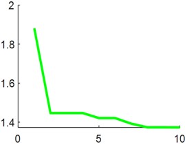
c) NGO minimum skewness square
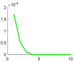
d) NGO minimum margin factor
Fig. 8Entropy values of different parameters
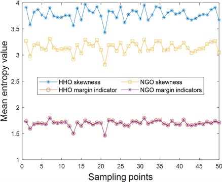
Second, the analysis of average entropy values for fault data underscores the critical role of the chosen objective function. When minimizing the squared skewness, entropy values were excessively high, indicating poor discrimination of fault information, which resulted in suboptimal parameter performance and significant entropy differences. In contrast, optimizing the minimum margin factor produced a much higher overlap in entropy values, with values that were more appropriate for fault feature extraction. This suggests superior parameter accuracy, leading to more effective dimensionality reduction and improved classification accuracy.
Therefore, although the similar experimental conditions led both HHO and NGO to achieve identical profit rate outcomes in this specific test, the entropy analysis clearly shows that the effectiveness of parameter optimization is fundamentally dependent on the choice of objective function. The minimum margin factor was found to be significantly more effective than the squared skewness for generating robust and informative parameters from the data.
By using a two-dimensional contour map, further examine the distribution of mean entropy values for 100 sample points of 10 types of faults.
Fig. 9Minimum skew square contour map
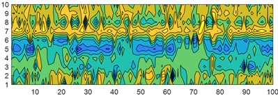
a) HHO minimum skewness square
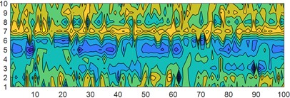
b) NGO minimum skewness square
Fig. 10Minimum margin factor contour map
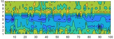
a) HHO minimum margin factor
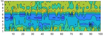
b) NGO minimum margin factor
It can be clearly seen from the graph that with the minimum skewness square as the objective function, the entropy values obtained by different optimization algorithms vary greatly, indicating that their performance as the objective function for optimization is not ideal; On the contrary, after extracting entropy information from the MRE parameters obtained with the minimum margin factor as the objective function, it can be seen that the fault characteristic signals of different optimization algorithms have minimal changes and almost no significant changes; At the same time, it can be found that the contour lines of the same type of horizontal faults obtained with the minimum skewness as the objective function are more encrypted, indicating that the entropy distribution obtained is wide, the data is discrete, and good fault information is not obtained; The entropy value obtained by the minimum margin factor is significantly more concentrated in the same fault category, indicating that the parameter effect obtained is better.
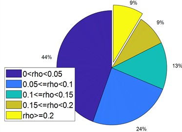
Further analyze the obtained 10 fault characteristic signals pairwise. Taking the results obtained by the NGO optimization algorithm as an example, compare the difference between the minimum skewness square and the minimum margin factor as objective functions through the distribution of Pearson correlation coefficients. Perform pairwise correlation tests on 10 types of fault characteristic signals, take the absolute value of the obtained correlation data, and classify it according to 0-0.05, 0.05-0.1, 0.1-0.15, 0.15-0.2, ≥ 0.2 to obtain Figs. 11, 12.
The dark blue area in the figure represents the proportion of the minimum correlation coefficient. It is evident from the figure that the MRE parameter obtained with the minimum margin factor as the objective function has a significantly larger proportion of the minimum correlation coefficient between the extracted fault feature signals than the minimum skewness square. The proportion of the dark blue area is as high as 44 %, indicating a high degree of discrimination in fault information.
There were ten types of original fault data, and the entire dataset size was 1000×128. The data was too large and the fault information was not clear enough, which not only was not conducive to subsequent classification, but also consumed too much time. Therefore, all fault category feature data with a size of 100×128 were subjected to dimensionality reduction using the ISOMAP manifold dimensionality reduction method [26], resulting in a data size of 100×32 after dimensionality reduction.
Fig. 11NGO skewness
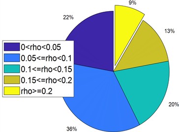
Fig. 12NGO margin factor
Taking the NGO optimization algorithm as an example, further compare the differences in fault signals extracted from MRE parameters obtained by different objective functions after dimensionality reduction. Select the feature data of 1000×32 of the fault feature signal set after dimensionality reduction for visualization processing, and obtain Figs. 13, 14.
Fig. 13NGO minimum margin factor scatter plot
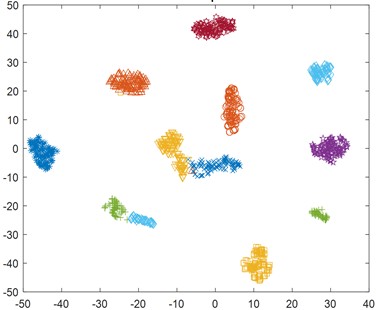
Fig. 14NGO minimum skewness squared scatter plot
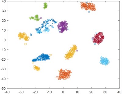
Through the visualization scatter plot of the data, it can be clearly seen that the discrimination of all feature data with the minimum margin factor is significantly better than the minimum skewness square. The fault feature signals of the same category are more concentrated, while the discrimination between different categories is more obvious and the overlap is low, which is beneficial for subsequent fault identification.
4. Analysis of identification results
The optimization algorithm of classifier DELM uniformly adopts NGO to classify the feature fault data after dimensionality reduction.
Combining the iterative curves of the four parameter optimization in Fig. 15, it can be seen that the starting point value of the NGO margin factor on the fitness value is lower and closer to the optimal fitness value. At the same time, it does not converge prematurely and may fall into local optima. This indicates that the fault feature information obtained by obtaining parameters through NGO margin factors is more accurate and has better discrimination.
The experimental results fully demonstrate the superiority and efficiency of NGO’s minimum margin factor in parameter optimization of MRE, whether in terms of fault identification accuracy and speed, or in the local optimization problem of convergence itself. The specific situation of NGO-DELM for identifying different parameters is shown in Fig. 16.
Fig. 15Iteration curve
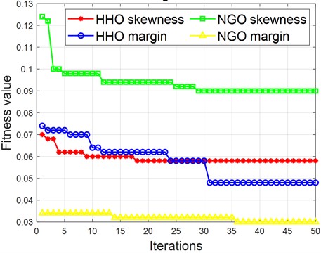
Table 3Identification results of the test set
Optimization method | Required time (s) | NGO-DLEM |
NGO minimum margin factor | 12.698815 | 97.8 % |
NGO minimum skewness square | 12.9925385 | 94.2 % |
HHO minimum margin factor | 13.1418923 | 97 % |
HHO minimum skewness square | 12.8209385 | 96.8 % |
It can be seen from the above table that the MRE parameters obtained after optimization with the NGO minimum margin factor have the highest recognition accuracy of fault feature signals after entropy value extraction, reaching 97.8 %, and the required time is the shortest, only 12.698815 seconds.
Fig. 16Confusion matrix: NGO-min margin factor
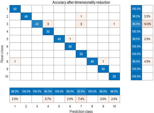
Fig. 17Confusion matrix: NGO-min skewness2
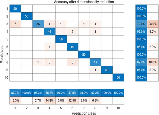
Fig. 18Confusion matrix: HHO-min margin factor
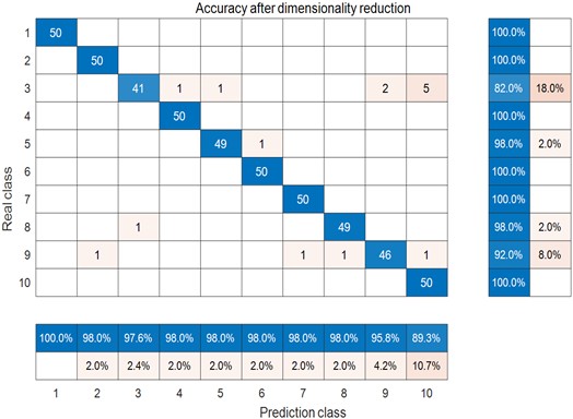
Fig. 19Confusion matrix: HHO-min skewness2

5. Conclusions
This paper proposes a fault diagnosis method based on Multi-scale Range Entropy (MRE) and a Deep Extreme Learning Machine (DELM), optimized by the Northern Goshawk Optimization (NGO) algorithm. This method effectively overcomes the problem of selecting MRE parameters based on manual experience. The experimental verification leads to the following quantitative conclusions:
1) The Choice of Objective Function is Critical: For selecting MRE parameters, using the minimum margin factor as the objective function yields superior results. The experimental results demonstrate that the NGO-minimum margin factor method achieved a fault recognition accuracy of 97.8 %, outperforming all other tested approaches. In contrast, using the “NGO-minimum skewness square” as the objective function resulted in a lower accuracy of 94.2 %. This demonstrates that the minimum margin factor is more effective in screening fault feature signals, ensuring the accuracy of the resulting fault information.
2) The NGO Algorithm Offers Superior Optimization Performance: The NGO optimization algorithm demonstrated outstanding performance in terms of both speed and accuracy. The proposed method not only achieved the highest accuracy but was also the fastest, completing the identification task in just 12.7 seconds. Furthermore, the fault feature information obtained was more effective. Pearson correlation analysis showed that features extracted using the minimum margin factor exhibited a high degree of discrimination, with the proportion of the minimum correlation coefficient reaching 44 %. The algorithm effectively avoids premature convergence and local optima, ensuring the reliability of the data in reflecting feature information.
References
-
J. Wang, L. Cui, and Y. Xu, “Quantitative and localization fault diagnosis method of rolling bearing based on quantitative mapping model,” Entropy, Vol. 20, No. 7, p. 510, Jul. 2018, https://doi.org/10.3390/e20070510
-
J. E. Qiu et al., “Bearing fault diagnosis based on self attention mechanism ACGAN,” Information and Control, 2023, https://doi.org/10.13976/j.cnki.xk.2022.2002
-
Z. Y. Wang and L. G. Yao, “Rolling bearing fault diagnosis method based on generalized refined composite multiscale sample entropy and manifold learning,” (in Chinese), China Mechanical Engineering, Vol. 31, No. 20, pp. 2463–2471, 2020, https://doi.org/10.3969/j.issn.1004-132x.2020.20.009
-
M. Pająk, Muślewski, B. Landowski, T. Kałaczyński, M. Kluczyk, and D. Kolar, “Identification of reliability states of a ship engine of the type Sulzer 6AL20/24,” SAE International Journal of Engines, Vol. 15, No. 4, pp. 527–542, Nov. 2021, https://doi.org/10.4271/03-15-04-0028
-
D. Zhao et al., “Parallel multi-scale entropy and it’s application in rolling bearing fault diagnosis,” Measurement, Vol. 168, p. 108333, Jan. 2021, https://doi.org/10.1016/j.measurement.2020.108333
-
X. Zhu, J. Zheng, H. Pan, J. Bao, and Y. Zhang, “Time-shift multiscale fuzzy entropy and Laplacian support vector machine based rolling bearing fault diagnosis,” Entropy, Vol. 20, No. 8, p. 602, Aug. 2018, https://doi.org/10.3390/e20080602
-
M. N. Yasir and B.-H. Koh, “Data decomposition techniques with multi-scale permutation entropy calculations for bearing fault diagnosis,” Sensors, Vol. 18, No. 4, p. 1278, Apr. 2018, https://doi.org/10.3390/s18041278
-
W. D. Jiao et al., “Multi-scale sample entropy-based energy moment features applied to fault classification,” IEEE Access, Vol. 2021, No. 9, pp. 8444–8454, 2021, https://doi.org/10.1109/access.2021.3050254
-
X. N. Zhang, C. H. Tang, and R. T. Zhou, “An adaptive morphological filtering algorithm and its application in bearing fault diagnosis,” (in Chinese), Journal of Xi’an Jiaotong University, Vol. 52, No. 12, pp. 1–8, Dec. 2018.
-
D. N. Chen, Y. D. Zhang, and C. Y. Yao, “Fault diagnosis of rolling bearings based on parameter optimization MPE and FCM,” (in Chinese), Bearing, Vol. 450, No. 5, pp. 33–38, May 2017.
-
H. Wang, Q. Li, S. Yang, and Y. Liu, “Fault recognition of rolling bearings based on parameter optimized multi-scale permutation entropy and Gath-Geva,” Entropy, Vol. 23, No. 8, p. 1040, Aug. 2021, https://doi.org/10.3390/e23081040
-
M. Zhang, “A fault diagnosis method for rolling bearings based on adaptive MCKD and VMD,” (in Chinese), Jiangxi University of Technology, Jiangxi, 2020.
-
J. Pi et al., “Application of BQGA-ELM network in fault diagnosis of rolling bearings,” (in Chinese), Vibration and Shock, Vol. 38, No. 18, pp. 192–200, 2019, https://doi.org/10.13465/j.cnki.jvs.2019.18.027
-
S. Tyagi and S. K. Panigrahi, “An improved envelope detection method using particle swarm optimisation for rolling element bearing fault diagnosis,” Journal of Computational Design and Engineering, Vol. 4, No. 4, pp. 305–317, Oct. 2017, https://doi.org/10.1016/j.jcde.2017.05.002
-
X. Fu et al., “Multi threshold image segmentation based on improved Northern Eagle algorithm,” (in Chinese), Computer Engineering, 2023, https://doi.org/10.19678/j.issn.1000-3428.0065186
-
M. Dehghani, S. Hubalovsky, and P. Trojovsky, “Northern goshawk optimization: a new swarm-based algorithm for solving optimization problems,” IEEE Access, Vol. 9, pp. 162059–162080, Jan. 2021, https://doi.org/10.1109/access.2021.3133286
-
G. X. Wang et al., “Bearing fault diagnosis based on multi-scale mean permutation entropy and parameter optimization support vector machine,” (in Chinese), Vibration and Shock, Vol. 41, No. 1, pp. 221–228, 2022, https://doi.org/10.13465/j.cnki.jvs.2022.01.028
-
W. F. Zhang, Z. C. Zhu, and D. H. Wu, “Rolling bearing fault diagnosis based on weighted domain adaptive convolutional neural network,” (in Chinese), Journal of System Simulation, 2023, https://doi.org/10.16182/j.issn1004731x.joss.22-0616
-
J. T. Song, S. X. Cui, and H. G. Liu, “Ultra short term wind power prediction based on quadratic decomposition of NGO VMD residual term and short-term memory neural network,” (in Chinese), Science and Technology and Engineering, Vol. 23, No. 6, pp. 2428–2437, Jun. 2023.
-
Y. H. Wang et al., “Transformer fault diagnosis method based on data equalization and improved whale algorithm optimizing kernel extreme learning machine,” (in Chinese), Information and Control, Vol. 52, No. 2, pp. 235–244, 2023, https://doi.org/10.13976/j.cnki.xk.2023.2112
-
W. S. Chen et al., “A bearing fault diagnosis method based on compressive sensing and improved deep limit learning machine,” (in Chinese), Mechanical Strength, Vol. 43, No. 4, pp. 779–785, 2021, https://doi.org/10.16579/j.issn.1001.9669.2021.04.003
-
S. Pang, X. Yang, X. Zhang, and Y. Sun, “Fault diagnosis of rotating machinery components with deep ELM ensemble induced by real-valued output-based diversity metric,” Mechanical Systems and Signal Processing, Vol. 159, p. 107821, Oct. 2021, https://doi.org/10.1016/j.ymssp.2021.107821
-
X. Zhao, M. Jia, J. Bin, T. Wang, and Z. Liu, “Multiple-order graphical deep extreme learning machine for unsupervised fault diagnosis of rolling bearing,” IEEE Transactions on Instrumentation and Measurement, Vol. 70, pp. 1–12, Jan. 2021, https://doi.org/10.1109/tim.2020.3041087
-
T. Han, J.-C. Gong, X.-Q. Yang, and L.-Z. An, “Fault diagnosis of rolling bearings using dual-tree complex wavelet packet transform and time-shifted multiscale range entropy,” IEEE Access, Vol. 10, pp. 59308–59326, Jan. 2022, https://doi.org/10.1109/access.2022.3180338
-
K. Li et al., “Fault diagnosis method based on improved deep limit learning machine,” (in Chinese), Vibration, Testing and Diagnosis, Vol. 40, No. 6, pp. 1120–1127, 1232, https://doi.org/10.16450/j.cnki.issn.1004-6801.2020.06.013
-
Z. C. Zhu, D. H. Wu, and Y. C. Yue, “Engine wear fault diagnosis based on supervised kernel entropy component analysis,” (in Chinese), Journal of System Simulation, Vol. 34, No. 1, pp. 45–52, 2022, https://doi.org/10.16182/j.issn1004731x.joss.20-0623
-
Y. Yang, H. Liu, L. Han, and P. Gao, “A feature extraction method using VMD and improved envelope spectrum entropy for rolling bearing fault diagnosis,” IEEE Sensors Journal, Vol. 23, No. 4, pp. 3848–3858, Feb. 2023, https://doi.org/10.1109/jsen.2022.3232707
About this article

The authors have not disclosed any funding.
The datasets generated during and/or analyzed during the current study are available from the corresponding author on reasonable request.
Feng Qihui: writing-original draft preparation, writing-review and editing. Liao Ziyang: data curation. Wang Jun: methodology. Chen Yongqi: conceptualization. Zhang Tao: software. Dai Qinge: formal analysis.
The authors declare that they have no conflict of interest.
