Abstract
Smart meters generate extensive data on individual consumer electricity usage, providing valuable insights that can aid in identifying demographic information and advancing the development of smart grids. Current research has primarily focused on traditional machine learning approaches for this task, with relatively few studies exploring deep learning methods, despite their potential for more accurate and efficient analysis. To address this gap, this paper proposes a self-supervised deep learning approach based on Convolutional Neural Network (CNN) to identify demographic information from smart meter data. The model leverages the Fast Fourier Transform (FFT) to detect frequency cycles within the dataset, which are then used to optimize the sizes of convolutional kernels. This design enhances periodic stability during shallow feature extraction, improving the model’s ability to capture meaningful patterns in the data. Furthermore, the model incorporates a self-supervised pre-training strategy to predict temporal and spatial interactions in load signals, effectively enhancing representation learning without relying on extensive labeled data. This approach ensures the model’s robustness and adaptability to different datasets. Comprehensive experiments were conducted on a publicly available Irish dataset to evaluate the model’s performance. Results demonstrate that the proposed model surpasses a series of state-of-the-art (SOTA) methods, achieving superior performance in demographic information identification. These findings highlight the effectiveness of integrating FFT-based kernel design and self-supervised learning in improving feature extraction and representation learning for smart meter data.
Highlights
- A self-supervised CNN framework integrating FFT-based adaptive convolutional kernels is proposed to identify demographic information from smart meter data, outperforming state-of-the-art methods in accuracy, recall, and F1-score across three tasks.
- The model leverages FFT to extract dominant periods from time series, which are used to optimize convolutional kernel sizes, enhancing periodic feature capture during shallow feature extraction and improving pattern recognition.
- A self-supervised pre-training strategy with contrastive learning on unlabeled data addresses limited labeled data challenges, enabling robust representation learning and superior performance in demographic identification tasks.
1. Introduction
Smart meters can collect extensive data on individual consumers’ electricity consumption [1-2]. By analyzing this data, it is possible to identify consumption patterns and sociodemographic information [3], which can help retailers provide more personalized services, optimize demand response, and promote the development of smart grids.
There has been prior work in the field of identifying sociodemographic information from load profiles. For instance, Beckel et al. [4] proposed a system called CLASS, achieving an accuracy of over 70 % through feature selection and classification. Hopf et al. [5] extended the CLASS system, designing 88 features and proposing a combined feature selection method. In [6], Viegas et al. used transparent fuzzy models to estimate consumer characteristics and extract knowledge. Zhong and Tam [7] combined the Discrete Fourier Transform with classification and regression trees to classify consumers. Wang et al. [8] used non-negative sparse coding to extract partial usage patterns and applied support vector machines to identify consumer types. While these traditional machine learning methods achieved promising results at the time, they have certain limitations. On the one hand, most methods require manual feature extraction, which is labor-intensive and resource-consuming. Moreover, handcrafted features often fail to fully capture the complex temporal and contextual dependencies in smart meter data, leading to suboptimal performance. On the other hand, despite their initial success, these methods still fall short in accuracy when compared to expert judgment.
In recent years, deep learning technologies have advanced rapidly, achieving significant progress in many tasks, such as time series analysis (including time series classification, forecasting, anomaly detection, etc.). For instance, when using time series data from smart meters as input and their corresponding demographic information as labels, the task of identifying demographic information from smart meter data can be framed as a time series classification problem. Consequently, methods used for deep learning-based time series classification can be effectively applied to demographic information identification. Unlike traditional machine learning methods, these deep learning approaches can analyze power load data without the need for manual feature extraction, fundamentally transforming the field of power load data classification. Although some recent studies have employed deep learning techniques to process power load time series data, much work remains to be done in this area. For example, autoencoders have been used in [11] to extract features from load curves. In [12, 13], a deep convolutional neural network was proposed to capture highly nonlinear relationships between electricity consumption at different times and dates and the demographic characteristics of consumers, identifying these characteristics based on automatically extracted features. However, there are still many directions to explore and unresolved challenges in this field. For instance, labeled smart meter datasets are scarce and difficult to obtain due to privacy concerns and the high cost of manual annotation. This scarcity of labeled data limits the effectiveness of supervised learning approaches and hinders the development of more accurate models. Additionally, the accuracy of existing deep learning-based models for power load data classification remains insufficient, as these models often require large-scale training data and suffer from overfitting when applied to small datasets.
In time series analysis, convolution plays a crucial role in balancing efficiency and performance. Models based on Temporal Convolutional Networks (TCNs) [14] have achieved good results in time series tasks. However, standard TCNs rely on fixed kernel sizes, limiting their adaptability to time series with varying periodic patterns. To address this, Modern Temporal Convolutional Networks (ModernTCN) [15] proposed using larger convolution kernels to expand the receptive field, improving performance in downstream tasks. Despite these advancements, existing methods still overlook the explicit integration of periodicity into convolution operations, which is essential for modeling recurring patterns in time series data. Additionally, periodic analysis is a powerful tool for identifying regular behaviors in time series. Prior works, such as [16], applied the Fast Fourier Transform (FFT) to time series data, leveraging frequency-domain sparsity to select the top K magnitudes and analyze their corresponding frequencies and periods. While effective, these approaches typically use frequency-domain information in isolation rather than integrating it directly into neural network architectures. Given that smart meter electricity load data exhibits strong periodicity, an approach that incorporates periodicity into the convolution process could further enhance classification performance. Furthermore, a key challenge in smart meter data analysis is the scarcity of labeled data. Existing deep learning models often rely on large labeled datasets, making them difficult to apply in real-world scenarios where labeled data is limited. Self-supervised learning (SSL) [17-19] presents a promising solution, enabling models to learn feature representations from unlabeled data. However, most SSL methods focus on time series forecasting or representation learning rather than classification tasks related to demographic information inference.
In light of the above discussion, this paper proposes a Convolutional Neural Network (CNN)-based framework with self-supervised learning to identify sociodemographic information from smart meter data [13]. Specifically, patch embedding operations are applied to the time series, generating -dimensional embedding vectors. Simultaneously, the input time series undergoes FFT to obtain the periods corresponding to the top magnitudes. The -dimensional embedding vectors are then subjected to depthwise separable convolution to extract temporal features, using the period lengths as the sizes of the convolution kernels. Unlike traditional TCNs with fixed kernels, this design dynamically adapts to the periodic characteristics of the data, allowing the network to learn more effective temporal patterns. Next, to further enhance feature extraction, two ConvFFN modules are introduced, which learn representations across variable and feature dimensions. This structure captures both local and global dependencies within the time series, improving classification performance. Finally, a classification module outputs the classification probabilities. Additionally, a self-supervised learning approach is utilized to pre-train the model on extensive unlabeled data, addressing the challenge of limited labeled data and enabling the acquisition of general feature representations. The model is then trained and fine-tuned on labeled data. Training was conducted on a publicly available smart meter dataset, with experimental results validated to demonstrate the effectiveness of the proposed method.
Our contributions can be summarized as follows:
– A self-supervised learning strategy is employed to address the limited labeled data challenge in sociodemographic information identification tasks utilizing smart meter data.
– By employing the top periods of the time series as kernel sizes in depthwise separable convolution, the periodicity of the time series is integrated with temporal convolution.
– Experimental results show that the proposed model outperforms a series of state-of-the-art (SOTA) models on the used dataset in classification tasks.
The rest of this paper is organized as follows. In Section 2, various time series classification methods and self-supervised learning approaches for time series are reviewed. The proposed network is detailed in Section 3. In Section 4, the experimental design is described, and the experimental results and analysis are presented. Finally, the paper is concluded in Section 5.
2. Related work
2.1. Deep learning-based methods for time series classification
In recent years, deep learning has made significant advancements in time series classification, largely due to the powerful feature learning capabilities of deep neural networks. Several methods have employed one-dimensional deep neural networks to achieve improved classification accuracy, such as Deep Residual Networks [20], Fully Convolutional Networks (FCN) [21], and InceptionTime [22]. Bouny et al. [23] proposed a model that uses CNNs and multi-scale fusion, achieving outstanding performance. Zhou et al. [24] designed a sparse self-attention mechanism and extraction operations to address the challenges of quadratic time complexity and memory usage in Transformers. Another study [25] developed an efficient self-correlation mechanism to discover dependencies and aggregate information at the sequence level. Additionally, [15] modernized the traditional TCNs by employing larger convolutional kernels, leading to the development of Modern TCN, which have demonstrated both excellent performance and efficiency in time series analysis tasks. Furthermore, [16] transformed one-dimensional time series data into two-dimensional space for analysis and proposed a task-generalized model called TimesNet, which has achieved SOTA results across five major time series analysis tasks including long-term forecasting, short-term forecasting, imputation, anomaly detection, and classification.
2.2. Self-supervised learning for time-series
Self-supervised learning (SSL) has emerged as a powerful paradigm for leveraging unlabeled data, particularly in the field of time series analysis [26-28]. Recent advancements in SSL have further demonstrated its effectiveness in various domains, including spectral analysis, remote sensing, and anomaly detection. For example, SpectralGPT [45] applies transformer-based architectures to spectral data modeling, capturing long-range dependencies effectively. SeaMo [46] introduces a multi-seasonal and multimodal approach, enabling robust self-supervised learning across diverse environmental conditions. Additionally, in hyperspectral analysis, disentangled prior learning [47] combines model-driven and data-driven paradigms to improve anomaly detection. These works highlight the increasing applicability of SSL in real-world time series scenarios, motivating further exploration in smart meter data analysis. Moreover, SSL techniques have garnered significant attention due to their ability to learn rich representations from raw time series data without requiring extensive manual labeling. Several methods have been proposed to harness the potential of SSL for time series data. One notable approach is contrastive learning. For example, SimCLR [29] replaced the momentum encoder with a larger number of negative pairs, while CPC [17] demonstrated the effectiveness of contrastive learning by predicting future time steps in the latent space, thereby enhancing model performance on downstream tasks. TS-TCC [19] designed time-series-specific augmentations to construct different views of the input data and introduced a novel cross-view temporal and contextual contrastive module to improve the learned representations. TS2Vec [30] introduced a hierarchical contrastive learning framework that captures both local and global temporal patterns by learning multi-scale representations. Another method, proposed in [31], involved sampling positive and negative pairs directly from the raw time series. It is worth noting that there are also some prototype-based time series contrastive learning methods. TapNet [32] introduced a learnable prototype for each predefined class, classifying input time series samples based on their distances to each class prototype. DVSL [33] introduced virtual sequences that function similarly to prototypes, minimizing the distance between samples and virtual sequences while maximizing the distance between different virtual sequences. Additionally, contrastive learning methods incorporating expert knowledge have been developed, where expert priors or information were integrated into deep neural networks to guide model training [34]. For example, SleepPriorCL [36] introduced prior features to ensure that the model correctly identifies positive and negative samples.
Another category of time series SSL methods is generative approaches, which primarily involve constructing generative tasks that enable the model to learn feature representations from time series data without labels. These methods include predicting future windows or specific timestamps using past sequences, reconstructing inputs via encoder-decoder architectures, and predicting unseen portions of masked time series. For example, THOC [37] constructed a multi-resolution single-step prediction self-supervised auxiliary task that allows the prediction task to be performed simultaneously at different resolutions by setting jump lengths. TimeMAE [38] randomly masked portions of data points in the time series and used a masked autoencoder to predict and reconstructed the masked data, thereby learning the latent feature representations of the time series.
Finally, adversarial methods also represent a common paradigm for self-supervised time series representation learning. TimeGAN [39], for instance, enhanced the time series generation framework by combining basic GANs with autoregressive models, preserving the dynamic characteristics of time series. PSA-GAN [40] introduced a self-attention mechanism within a framework designed for long time series generation.
These SSL methods for time series have shown significant promise in improving the accuracy and generalization of tasks such as classification, forecasting, and anomaly detection [42, 43]. As SSL techniques continue to evolve, they are expected to play an increasingly important role in time series analysis, offering a scalable solution to the challenges posed by limited labeled data.
3. Methods
3.1. Overall framework
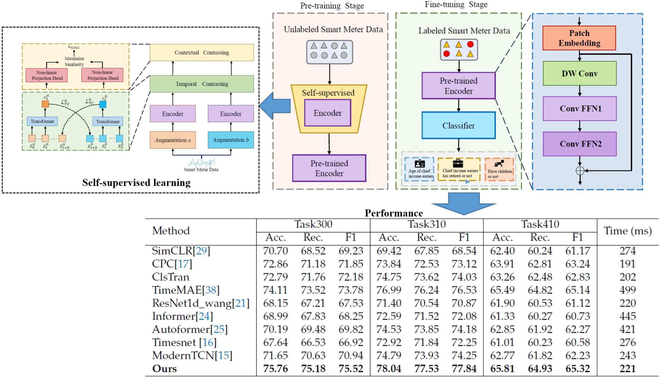
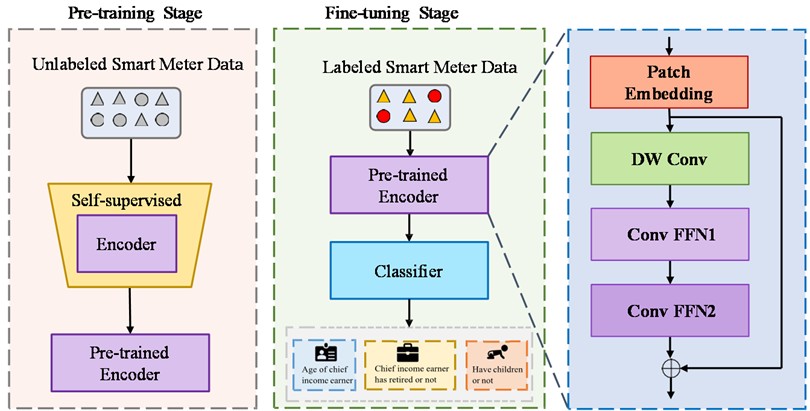
This paper focuses on user behavior analysis in smart meter data. The overall architecture of the proposed network is shown in Fig. 1. The model is divided into two stages: pre-training and fine-tuning. In the pre-training stage, a large amount of unlabeled data is used for training to complete the self-supervised task based on the contrastive learning method. In the fine-tuning stage, the pre-trained encoder is used to perform fine-tuning training on labeled data. The encoder first performs patching and embedding operations on the input time series to obtain a -dimensional embedding vector. Then, this vector is passed to the deep convolution module to extract the time dimension information. A large kernel is used in the DWConv module to increase the receptive field. In order to combine the periodicity of the time series with the temporal convolution, the cycles obtained by FTT on the input sample are used as the kernel size of the convolution operation. Subsequently, two ConvFFN modules are applied to extract information from the feature and variable dimensions, respectively. The obtained feature representation is then input to the classification layer. The following subsections provide a detailed description of each process.
Fig. 1Overview of the proposed model. The model is divided into two stages: pre-training and fine-tuning. In the pre-training stage, the model is trained using unlabeled data, while in the fine-tuning stage, labeled data is used. The encoder consists of a patching embedding module, a Depthwise Convolution (DW Conv) module, and two ConvFFN modules. The DW Conv module is responsible for extracting information along the time dimension. The ConvFFN1 and ConvFFN2 modules are responsible for extracting feature and variable dimension information, respectively. Finally, the classification layer outputs the classification results
3.2. Network architecture details
3.2.1. FFT
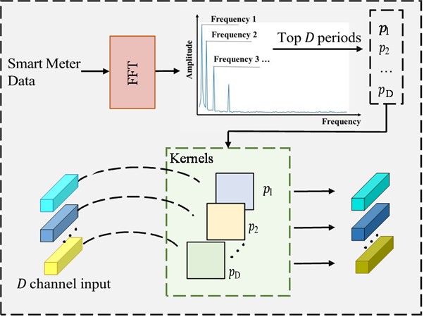
Applying the FFT to time series data allows us to obtain its frequency spectrum, which in turn enables the identification of dominant periods through frequency domain analysis. This approach is both common and critical in time series analysis, as it helps uncover periodic or recurrent patterns within the data. In the resulting frequency spectrum, peaks with higher amplitudes indicate that those frequencies play a more significant role in the original time series. Specifically, Considering a univariate smart meter time series , where represents the length, FFT is employed to analyze the series in the frequency domain. The process can be outlined as follows:
where, and denote the FFT and the calculation of amplitude values. represents the calculated amplitude of each frequency. Considering the sparsity in the frequency domain and to avoid noise from irrelevant high-frequency components , only the top amplitudes are selected, enabling identification of the most significant frequencies , where is equal to the dimensionality of the embedding vector obtained after the time series passes through the Patching and Embedding layer in the lower branch. The corresponding period lengths for these frequencies are .
3.2.2. Patch embedding
For the input smart meter time series , padding is first applied, followed by segmentation into overlapping patches, each of size . The stride of the patching process is set to . These patches are then embedded into -dimensional embedding vectors:
where PE refers to the Patching and Embedding operation, is the input embedding.
3.2.3. DWConv
As is shown in Fig. 2, DWConv is a combination of depthwise convolution and pointwise convolution that significantly reduces computational complexity and the number of parameters. Specifically, after the initial Patching and Embedding operations, the time series data is transformed into . In DWConv, the feature and variable channels are independent, with each channel learning the temporal dependencies separately. The number of convolution channels is set to 1× to extract features along the temporal dimension. Inspired by the approach in modernTCN [13], large kernels are used to expand the receptive field and enhance the model’s ability to capture temporal dependencies. To better leverage the periodic nature of time series data, the period lengths derived from FFT are proposed as kernel sizes for the convolutional filters in DWConv. This integration of periodicity into the convolution process is expected to improve model performance.
Fig. 2The structure of DW
3.2.4. ConvFFN
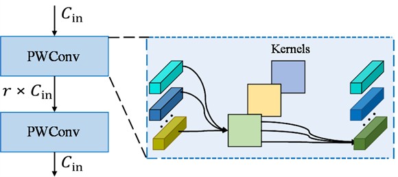
The ConvFFN comprises two modules, ConvFFN1 and ConvFFN2. As depicted in Fig. 3, each module consists of two pointwise convolution (PWConv) layers and adopts an inverted bottleneck structure, where the hidden channels in the ConvFFN block are expanded to be times wider than the input channels. Each ConvFFN module is designed to mix information from either the variable or feature dimensions exclusively, a decoupling design that reduces computational complexity and enhances model performance. Both ConvFFN modules utilize group convolution, with the number of groups set to the number of channels, meaning each group has only one channel. Specifically, in ConvFFN1, the number of variables is treated as the number of groups, allowing for the extraction of feature dimension information. Similarly, in ConvFFN2, the output from ConvFFN1 is transposed, treating the number of features as the number of groups to extract variable dimension information. To facilitate the training of deeper neural networks and improve the model’s generalization ability, residual connections are employed, linking the input embedding with the output of ConvFFN2.
Fig. 3Structure of ConvFFN
3.3. Self-supervised learning framework
To address the challenge of limited labeled smart meter data, a self-supervised learning approach is employed, leveraging a large amount of unlabeled data to pre-train the model. Following the method in [17], a self-supervised learning framework is designed, as shown in Fig. 4. For the input smart meter time series, both strong augmentation (augmentation ) and weak augmentation (augmentation ) are applied, generating two distinct but related views. The Encoder module in the figure represents the proposed model, which completes a view prediction task during the pre-training phase. Subsequently, a temporal contrastive module and a contextual contrastive module are introduced to maximize temporal and contextual consistency across the model’s outputs. Each module will be discussed in detail later.
3.3.1. Data augmentation
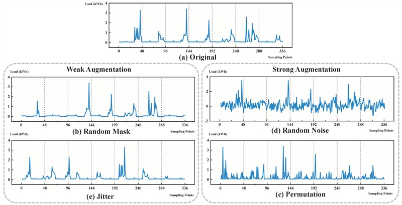
Data augmentation plays a critical role in contrastive learning [29, 44]. By generating different views of the same data sample, data augmentation enables the model to learn more robust feature representations. During contrastive learning, the model seeks to maximize the similarity between different views of the same sample while minimizing its similarity with other samples. This approach helps the model better capture the intrinsic characteristics of the data, thereby enhancing its generalization ability and robustness. Thus, designing effective data augmentations is essential. Specifically, for a given smart meter time series sample , a strong augmentation module and a weak augmentation module generate a strongly augmented view and a weakly augmented view , respectively. The strong augmentation operations include adding random noise and permutation. The weak augmentation strategy applies random mask and jitter. A comparison of the time series after both augmentations with the original sequence is presented in Fig. 5. These augmented views and are then fed into the Encoder module (which represents the proposed model), producing high-dimensional latent representations and . These high-dimensional representations are subsequently input into the temporal contrastive module.
Fig. 4Overall architecture of Self-supervised learning. The self-supervised learning framework primarily consists of two components. In the temporal contrastive module, a rigorous cross-view prediction task is designed to learn robust representations from the time series data. Building on these robust representations, the contextual contrastive module further enables the model to learn discriminative features
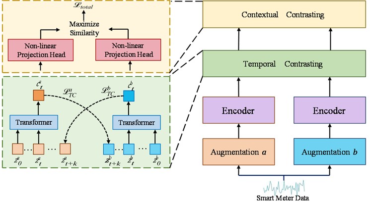
Fig. 5The original time series and the four argument time series
3.3.2. Temporal contrasting
The input to the temporal contrast module consists of the high-dimensional latent representations and generated by the encoder, with the output being the corresponding context vectors and . In this module, a cross-view prediction task is designed: the context vector is used to predict the future time steps () of , and conversely, the context vector is used to predict the future time steps of . To accomplish this prediction task, a log-bilinear model is employed to map back to the same dimensionality as , thereby preserving the mutual information between and . Next, a contrastive loss is applied to maximize the dot product between the predicted representation and the true representation of the same sample, while minimizing the dot product with representations of other samples within the mini-batch . The temporal contrastive loss proposed in [19] is adopted, which includes the following two types of contrastive losses:
3.3.3. Contextual contrasting
The contextual contrastive module maps contexts into a space where contextual contrastive learning is applied, with the goal of encouraging the model to learn more discriminative representations. Specifically, given a batch of input samples, augmentation produces 2 augmented views, resulting in 2 contexts. For a context , is denoted as the positive sample of , where the positive sample comes from the other augmented view of the same input. Hence, is considered a positive pair. Negative samples are drawn from the remaining 2-2 contexts within the same batch from other inputs, meaning that can form 2-2 negative pairs with its negative samples. The contextual contrastive loss is then designed to maximize the similarity between the sample and its positive pair while minimizing its similarity with the negative samples within the mini-batch. In this work, the contextual contrastive loss proposed in is adopted. The loss function is formulated as follows:
where denotes the dot product between normalized and , , represents the temperature coefficient.
The overall self-supervised loss is a weighted sum of two temporal contrastive losses and the contextual contrastive loss, as shown below:
where and are fixed scalar hyperparameters denoting the relative weight of each loss.
4. Experimental design
4.1. Dataset
The Irish Smart Meter Customer Behavior Trial dataset was provided by the Commission for Energy Regulation (CER), the regulatory authority for the electricity and gas sectors in Ireland. This dataset includes smart meter data from 4,232 residential users, with electricity usage recorded at 30-minute intervals over a period of 536 days. In addition, each resident completed a questionnaire containing over 200 questions. For this experiment, the data was segmented on a weekly basis, resulting in an effective dimension of 336 for each sample. After cleaning the data to remove samples with missing values, approximately 310,000 weeks of smart meter data remained. Of this, 80 % was allocated to the training set, and the remaining 20 % was used as the test set.
Table 1Dataset introduction
Question No. | Question | Answer | Number |
300 | Age of chief income earner | Young (< 35) | 33136 |
Medium (35-65) | 214244 | ||
Old (> 65) | 72428 | ||
310 | Chief income earner has retired or not | Yes | 97660 |
No | 223972 | ||
410 | Have children or not | Yes | 93404 |
No | 228228 |
Three survey questions in the dataset were selected based on their quantifiability to serve as tasks for this experiment. The specific details are shown in Table 3. These tasks leverage the dataset’s demographic annotations to explore how energy consumption patterns correlate with household attributes
Task300: Classifying the age group of the chief income earner (Young: < 35 years, Medium: 35-65 years, Old: > 65 years). Age is a critical factor in energy consumption, as it influences lifestyle patterns – e.g., working-age households (Medium) may exhibit peak usage in evenings, while older households (Old) may use more energy during the day. This task was selected to test the model’s ability to capture age-related consumption differences, which are essential for tailoring energy services to diverse age groups.
Task310: Determining whether the chief income earner has retired (Yes/No). Retirement status affects daily routines, with retired households potentially showing more consistent daytime usage compared to the variable patterns of working households. This task was selected because it challenges the model to detect subtle shifts in consumption linked to employment status, a key demographic variable for energy demand forecasting.
Task410: Identifying whether the household has children (Yes/No). The presence of children increases energy use due to additional appliance usage, heating, and cooling needs. This task was included to evaluate the model’s capacity to recognize high-variability consumption patterns, which are significant for family-oriented energy policies and load balancing in smart grids.
4.2. Comparison models
4.2.1. Self-supervised model
SimCLR: An unsupervised contrastive learning method based on data augmentation, originally developed in the field of computer vision.
CPC: a contrastive self-supervised learning method that focuses on predicting future time steps.
CLSTRAN: a multi-input unsupervised contrastive learning method.
TimeMAE: a representation learning method based on feature masking and reconstruction.
4.2.2. Universal time series representation learning model
ResNet1D-Wang: a classical one-dimensional fully convolutional residual network architecture.
Informer: a parallel multi-kernel feature extractor inspired by the Inception architecture, modified to process one-dimensional data effectively.
Autoformer: a long-term time series representation learning model based on a deep decomposition framework and auto-correlation mechanisms.
TimesNet: a model that adaptively transforms time series data into two-dimensional representations for comprehensive feature extraction.
ModernTCN: a pure convolutional architecture that employs extremely large convolutional kernels for enhanced temporal feature learning.
4.3. Implementation details
For the feature extraction process, a deep learning-based approach utilizing backpropagation gradient training is employed to automatically extract hierarchical features from the raw data. This process leverages the proposed model’s multi-layer neural network architecture, where each successive layer learns progressively more abstract representations of the input data. This stands in contrast to traditional machine learning approaches that rely on manually engineered feature extraction. To ensure experimental fairness, all baseline models included in our comparison similarly adopt this deep learning paradigm for feature extraction, thereby maintaining methodological consistency across our evaluation framework.
Both the pre-training and fine-tuning processes were conducted for 60 epochs, with a batch size of 128. The Adam optimizer was used with a learning rate of 3e-4, along with a weight decay strategy. All experiments were implemented using PyTorch 2.2.1 and trained on an NVIDIA GeForce RTX 4090 Ti GPU.
4.4. Evaluation metrics
To evaluate the performance of the model, three key metrics are used. Accuracy measures the proportion of correctly classified samples. Recall quantifies the model’s ability to identify all relevant instances of a class. Finally, F1 Score balances precision and recall to provide a comprehensive measure of model performance, particularly in imbalanced datasets.
4.5. Experimental results
4.5.1. Compared with previous models
Comprehensive comparisons between the proposed model and previous approaches were conducted, with detailed quantitative results systematically presented in Table 2. The experimental evaluation demonstrates that the proposed model consistently maintains superior performance across all evaluation tasks. Specifically, compared to general time-series representation learning models, our proposed model achieves significant improvements over the suboptimal model, with accuracy increasing by 4.11 %, 3.25 %, and 2.96 % on Task300, Task310, and Task410 respectively; recall improving by 4.55 %, 3.6 %, and 3.01 %; and F1-score enhancing by 4.58 %, 3.59 %, and 3.05 %. These substantial improvements are primarily attributed to the proposed model’s enhanced representation learning capability for smart meter signals, achieved through an innovative pre-training strategy that effectively captures the unique characteristics of energy consumption patterns.
When compared with previously proposed self-supervised models, our architecture demonstrates distinct structural advantages in feature extraction. The key innovation lies in our adaptive convolutional kernel design, which dynamically adjusts its receptive field to better capture both short-term fluctuations and long-term periodic dependencies in smart meter data. This architectural superiority translates into consistent performance gains over the suboptimal self-supervised model TimeMAE, with accuracy improvements of 1.65 %, 1.05 %, and 0.32 %; recall enhancements of 1.66 %, 1.29 %, and 0.11 %; and F1-score increases of 1.74 %, 1.31 %, and 0.18 % across the three evaluation tasks respectively. These results not only validate the effectiveness of our model design but also highlight the critical importance of incorporating pre-training strategies when addressing the challenging task of demographic information identification from smart meter data, where signal patterns are typically subtle and highly variable.
Table 2Performance on Task-300, Task-310, and Task-410
Method | Task300 | Task310 | Task410 | Time (ms) | ||||||
Acc. | Rec. | F1 | Acc. | Rec. | F1 | Acc. | Rec. | F1 | ||
SimCLR | 70.70 | 68.52 | 69.23 | 69.42 | 67.85 | 68.54 | 62.40 | 60.24 | 61.17 | 274 |
CPC | 72.86 | 71.18 | 71.85 | 73.84 | 72.53 | 73.12 | 63.91 | 62.81 | 63.24 | 191 |
ClsTran | 72.79 | 71.76 | 72.18 | 74.75 | 73.62 | 74.03 | 63.26 | 62.48 | 62.83 | 202 |
TimeMAE | 74.11 | 73.52 | 73.78 | 76.99 | 76.24 | 76.53 | 65.49 | 64.82 | 65.14 | 499 |
ResNet1d_wang | 68.15 | 67.21 | 67.53 | 71.40 | 70.54 | 70.87 | 61.90 | 60.53 | 61.12 | 220 |
Informer | 68.99 | 67.83 | 68.25 | 72.59 | 71.52 | 72.08 | 61.33 | 60.27 | 60.73 | 445 |
Autoformer | 70.19 | 69.48 | 69.82 | 74.53 | 73.85 | 74.18 | 62.85 | 61.92 | 62.27 | 421 |
Timesnet | 67.64 | 66.53 | 66.92 | 72.92 | 71.84 | 72.25 | 61.01 | 60.23 | 60.58 | 276 |
ModernTCN | 71.65 | 70.63 | 70.94 | 74.79 | 73.93 | 74.25 | 62.77 | 61.82 | 62.23 | 243 |
Ours | 75.76 | 75.18 | 75.52 | 78.04 | 77.53 | 77.84 | 65.81 | 64.93 | 65.32 | 221 |
Additionally, inference speed tests were conducted for various models, with the time values presented in the table corresponding to the inference duration per 100 samples. As can be observed, our proposed model demonstrates superior inference efficiency. Compared to Transformer-based architectures, the CNN-based structure exhibits fewer parameters and benefits from more optimized low-level implementations.
4.5.2. Ablation studies
In order to demonstrate the impact of adaptive convolution kernels on model performance and the performance improvement brought by super large convolution kernels at different locations, experiments were conducted on Task300, Task310, and Task410. The results are shown in Table 3.
Table 3Comparison of performance using large convolution kernels at different locations
Method | Task300 | Task310 | Task410 | ||||||
Acc. | Rec. | F1 | Acc. | Rec. | F1 | Acc. | Rec. | F1 | |
ModernTCN | 71.39 | 70.63 | 70.94 | 74.92 | 73.93 | 74.25 | 62.84 | 61.82 | 62.23 |
First block | 75.79 | 75.18 | 75.52 | 78.06 | 77.53 | 77.84 | 65.80 | 64.93 | 65.32 |
Second block | 74.46 | 73.85 | 74.20 | 77.12 | 76.64 | 76.92 | 64.75 | 63.88 | 64.27 |
Third block | 72.11 | 71.42 | 71.75 | 75.23 | 74.72 | 75.03 | 63.45 | 62.57 | 62.96 |
Fourth block | 70.49 | 69.95 | 70.28 | 73.68 | 73.15 | 73.46 | 62.12 | 61.24 | 61.63 |
First and Second block | 72.77 | 72.13 | 72.46 | 75.94 | 75.42 | 75.73 | 63.88 | 63.01 | 63.40 |
Experimental results indicate that using adaptive-sized convolutional kernels in the first block significantly improves accuracy across all tasks. For example, on Task300, the model with adaptive kernels in the first block achieves an accuracy of 75.77 %, compared to 71.51 % for the baseline model (ModernTCN). Similar improvements are observed on Task310 (78.06 % vs. 74.92 %) and Task410 (65.80 % vs. 62.84 %). This suggests that the early layers of the model play a crucial role in capturing periodic features, which are essential for accurate predictions.
However, as the model depth increases, the effectiveness of larger convolutional kernels diminishes. For instance, applying adaptive kernels in the third block results in lower accuracy compared to the first block (72.01 % vs. 75.77 % on Task300). This is likely because features in deeper layers become more abstract, and their inherent periodic characteristics are less pronounced. Consequently, the use of extremely large convolutional kernels in later blocks becomes less meaningful.
Furthermore, due to the constraints of input sequence length, adaptive-sized convolutional kernels can only be applied simultaneously in the first and second blocks at most. While this configuration improves accuracy compared to the baseline (72.72 % vs. 71.51 % on Task300), it underperforms compared to using adaptive kernels solely in the first block (72.72 % vs. 75.77 %). This further underscores the importance of the first block in capturing critical periodic features.
Table 4The size of the convolutional kernels provided by different extraction methods.
Method | Kernel size |
ACF | [3. 7. 9. 11.] |
HHT | [367. 104. 49. 19.] |
PD | [3. 4. 7. 14] |
WT | [5. 68. 57. 39.] |
FFT | [42. 36. 44. 34.] |
To demonstrate the impact of different time series periodicity extraction methods on the guidance of subsequent representation learning, several non-learning techniques were employed and tested across three tasks. Specifically, the Autocorrelation Function (ACF), Hilbert-Huang Transform (HHT), Peak Detection (PD), Wavelet Transform (WT), and Fast Fourier Transform (FFT) were utilized. The results are presented in the accompanying Fig. 6 and Tabel 4.
Fig. 6The impact of different extraction methods on the final classification results.
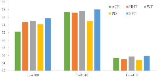
FFT achieved the highest accuracy across all three tasks, followed by WT, while ACE and PD exhibited poor performance. By comparing the sizes of the convolutional kernels introduced by these methods, it appears that using larger kernels may be a crucial strategy for enhancing accuracy.
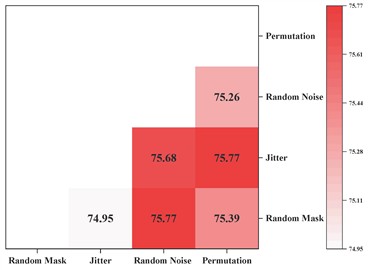
Contrastive self-supervised learning is a key step in improving the proposed model’s performance. To explore the impact of different data augmentation combinations on self-supervised learning performance in smart meter data, pairwise combinations of the four methods shown in Fig. 5 were evaluated across three datasets. The experimental results are shown in Fig. 7. It can be observed that “random noise + random mask” and “Permutation + Jitter” achieve the highest performance in Task300, with "Permutation + Jitter" yielding the best performance in Task310, and “random noise + Jitter” achieving the best performance in Task400. Analysis reveals that applying strong and weak augmentation on the two branches of contrastive learning is the best strategy. This is because different intensities of feature augmentation contain latent information at varying granularities, which requires the model to have stronger feature extraction capabilities to achieve the contrastive learning objective.
Fig. 7The impact of different data augmentation combinations on the final classification results.
a) Task300
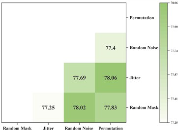
b) Task310
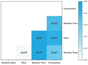
c) Task410
5. Conclusions
This paper proposes a CNN-based self-supervised learning approach to address the task of identifying demographic information from smart meter data. The proposed architecture utilizes the FFT to identify frequency cycles within the dataset, which are then used to determine the convolutional kernel size. This method enhances periodic stability during shallow feature extraction, thereby improving the model’s feature extraction capabilities. Additionally, the model is pre-trained in a self-supervised manner, enhancing its ability to learn representations of load signals through temporal and spatial interaction prediction. The superiority of our proposed architecture is demonstrated across three experiments, supporting the effectiveness of combining self-supervised pre-training with fine-tuning, along with a scientifically designed load signal extraction structure, as a viable solution for this task.
The practical implications of this work are significant. Smart meter data, which captures nuanced patterns in electricity usage, serves as a valuable resource for identifying demographic traits such as age, employment status, and household composition. Our model effectively distinguishes, for instance, the consumption behaviors of young, middle-aged, and older chief income earners, as well as detects signatures of retirement or the presence of children in a household. These insights are grounded in the model’s ability to extract and interpret periodic and behavioral features from the data, as validated by our experimental outcomes. Beyond demographic identification, this user behavior analysis holds transformative potential for smart grid development. Utilities can leverage these demographic insights to design targeted demand response programs, energy efficiency initiatives, and dynamic pricing strategies tailored to specific consumer segments. For example, understanding the age or employment status of households enables more precise load forecasting and grid management, enhancing the efficiency and reliability of smart grids. These advancements pave the way for more responsive and sustainable energy systems.
However, key challenges remain in smart meter data analysis, including privacy and security concerns, the need for robust, generalizable models, and dataset limitations in capturing long-term trends. Future research should focus on privacy-preserving frameworks, enhancing model interpretability, leveraging self-supervised and transfer learning, and integrating multi-source data for richer behavioral analysis.
References
-
Y. Wang et al., “Load profiling and its application to demand response: A review,” Tsinghua Science and Technology, Vol. 20, No. 2, pp. 117–129, Apr. 2015, https://doi.org/10.1109/tst.2015.7085625
-
F. Yang, X. Hou, G. Pan, Q. Luo, and C. Huang, “Research on reliability modeling and evaluation method of smart meter,” in IEEE International Conference on Automation, Electronics and Electrical Engineering (AUTEEE), pp. 244–248, Nov. 2018, https://doi.org/10.1109/auteee.2018.8720801
-
C. Beckel, L. Sadamori, T. Staake, and S. Santini, “Revealing household characteristics from smart meter data,” Energy, Vol. 78, pp. 397–410, Dec. 2014, https://doi.org/10.1016/j.energy.2014.10.025
-
C. Beckel, L. Sadamori, and S. Santini, “Automatic socio-economic classification of households using electricity consumption data,” in 4th International Conference on Future Energy Systems, pp. 75–86, May 2013, https://doi.org/10.1145/2487166.2487175
-
K. Hopf, M. Sodenkamp, I. Kozlovkiy, and T. Staake, “Feature extraction and filtering for household classification based on smart electricity meter data,” Computer Science – Research and Development, Vol. 31, No. 3, pp. 141–148, Nov. 2014, https://doi.org/10.1007/s00450-014-0294-4
-
J. L. Viegas, S. M. Vieira, and J. M. C. Sousa, “Mining consumer characteristics from smart metering data through fuzzy modelling,” in 16th International Conference on Information Processing and Management of Uncertainty in Knowledge-Based Systems, 2016.
-
S. Zhong and K.-S. Tam, “Hierarchical classification of load profiles based on their characteristic attributes in frequency domain,” IEEE Transactions on Power Systems, Vol. 30, No. 5, pp. 2434–2441, Sep. 2015, https://doi.org/10.1109/tpwrs.2014.2362492
-
Y. Wang, Q. Chen, C. Kang, Q. Xia, and M. Luo, “Sparse and redundant representation-based smart meter data compression and pattern extraction,” IEEE Transactions on Power Systems, Vol. 32, No. 3, pp. 2142–2151, May 2017, https://doi.org/10.1109/tpwrs.2016.2604389
-
Y. Lecun, Y. Bengio, and G. Hinton, “Deep learning,” Nature, Vol. 521, No. 7553, pp. 436–444, May 2015, https://doi.org/10.1038/nature14539
-
G. E. Hinton and R. R. Salakhutdinov, “Reducing the dimensionality of data with neural networks,” Science, Vol. 313, No. 5786, pp. 504–507, Jul. 2006, https://doi.org/10.1126/science.1127647
-
E. D. Varga, S. F. Beretka, C. Noce, and G. Sapienza, “Robust real-time load profile encoding and classification framework for efficient power systems operation,” IEEE Transactions on Power Systems, Vol. 30, No. 4, pp. 1897–1904, Jul. 2015, https://doi.org/10.1109/tpwrs.2014.2354552
-
Y. Wang, Q. Chen, D. Gan, J. Yang, D. S. Kirschen, and C. Kang, “Deep learning-based socio-demographic information identification from smart meter data,” IEEE Transactions on Smart Grid, Vol. 10, No. 3, pp. 2593–2602, May 2019, https://doi.org/10.1109/tsg.2018.2805723
-
J. Song et al., “Short-term wind power prediction based on deviation compensation TCNLSTM and step transfer strategy,” Southern Power System Technology, Vol. 17, No. 12, pp. 71–79, 2023.
-
S. Bai, J. Z. Kolter, and V. Koltun, “An empirical evaluation of generic convolutional and recurrent networks for sequence modeling,” arXiv:1803.01271, Mar. 2018, https://doi.org/1803.01271
-
D. Luo and X. Wang, “Moderntcn: A modern pure convolution structure for general time series analysis,” in The Twelfth International Conference on Learning Representations, 2024.
-
H. Wu, T. Hu, Y. Liu, H. Zhou, J. Wang, and M. Long, “TimesNet: temporal 2D-variation modeling for general time series analysis,” in International Conference on Learning Representations, Jan. 2022, https://doi.org/10.48550/arxiv.2210.02186
-
A. Oord, Y. Li, and O. Vinyals, “Representation learning with contrastive predictive coding,” arXiv: 1807.03748, Jan. 2018, https://doi.org/10.48550/arxiv.1807.03748
-
E. Eldele et al., “Time-series representation learning via temporal and contextual contrasting,” in 13th International Joint Conference on Artificial Intelligence {IJCAI-21}, pp. 2352–2359, Aug. 2021, https://doi.org/10.24963/ijcai.2021/324
-
E. Eldele et al., “Self-supervised contrastive representation learning for semi-supervised time-series classification,” IEEE Transactions on Pattern Analysis and Machine Intelligence, Vol. 45, No. 12, pp. 15604–15618, Dec. 2023, https://doi.org/10.1109/tpami.2023.3308189
-
T. He, Z. Zhang, H. Zhang, Z. Zhang, J. Xie, and M. Li, “Bag of tricks for image classification with convolutional neural networks,” in IEEE/CVF Conference on Computer Vision and Pattern Recognition (CVPR), pp. 558–567, Jun. 2019, https://doi.org/10.1109/cvpr.2019.00065
-
Z. Wang, W. Yan, and T. Oates, “Time series classification from scratch with deep neural networks: A strong baseline,” in International Joint Conference on Neural Networks (IJCNN), pp. 1578–1585, May 2017, https://doi.org/10.1109/ijcnn.2017.7966039
-
H. Ismail Fawaz et al., “InceptionTime: finding AlexNet for time series classification,” Data Mining and Knowledge Discovery, Vol. 34, No. 6, pp. 1936–1962, Sep. 2020, https://doi.org/10.1007/s10618-020-00710-y
-
X. Fan, Q. Yao, Y. Cai, F. Miao, F. Sun, and Y. Li, “Multiscaled fusion of deep convolutional neural networks for screening atrial fibrillation from single lead short ECG recordings,” IEEE Journal of Biomedical and Health Informatics, Vol. 22, No. 6, pp. 1744–1753, Nov. 2018, https://doi.org/10.1109/jbhi.2018.2858789
-
H. Zhou et al., “Informer: Beyond efficient transformer for long sequence time-series forecasting,” in Proceedings of the AAAI Conference on Artificial Intelligence, Vol. 35, No. 12, pp. 11106–11115, May 2021, https://doi.org/10.1609/aaai.v35i12.17325
-
H. Wu, J. Xu, J. Wang, and M. Long, “Autoformer: decomposition transformers with auto-correlation for long-term series forecasting,” arXiv:2106.13008, pp. 101–112, Jan. 2021, https://doi.org/10.48550/arxiv.2106.13008
-
G.-J. Qi and J. Luo, “Small data challenges in big data era: a survey of recent progress on unsupervised and semi-supervised methods,” arXiv:1903.11260, Jan. 2019, https://doi.org/10.48550/arxiv.1903.11260
-
L. Jing and Y. Tian, “Self-supervised visual feature learning with deep neural networks: a survey,” IEEE Transactions on Pattern Analysis and Machine Intelligence, Vol. 43, No. 11, pp. 4037–4058, Nov. 2021, https://doi.org/10.1109/tpami.2020.2992393
-
A. Jaiswal, A. R. Babu, M. Z. Zadeh, D. Banerjee, and F. Makedon, “A survey on contrastive self-supervised learning,” Technologies, Vol. 9, No. 1, Dec. 2020, https://doi.org/10.3390/technologies9010002
-
T. Chen, S. Kornblith, M. Norouzi, and G. Hinton, “A simple framework for contrastive learning of visual representations,” arXiv:2002.05709, Jan. 2020, https://doi.org/10.48550/arxiv.2002.05709
-
Z. Yue et al., “TS2Vec: towards universal representation of time series,” arXiv:2106.10466, Jan. 2021, https://doi.org/10.48550/arxiv.2106.10466
-
J.-Y. Franceschi, A. Dieuleveut, and M. Jaggi, “Unsupervised scalable representation learning for multivariate time series,” arXiv:1901.10738, Vol. 32, Jan. 2019, https://doi.org/10.48550/arxiv.1901.10738
-
X. Zhang, Y. Gao, J. Lin, and C.-T. Lu, “Tapnet: multivariate time series classification with attentional prototypical network,” in Proceedings of the AAAI Conference on Artificial Intelligence, Vol. 34, No. 4, pp. 6845–6852, Apr. 2020, https://doi.org/10.1609/aaai.v34i04.6165
-
A. Dorle, F. Li, W. Song, and S. Li, “Learning discriminative virtual sequences for time series classification,” in Proceedings of the 29th ACM International Conference on Information and Knowledge Management, pp. .2001–2004, 2020.
-
X. Wu, L. Xiao, Y. Sun, J. Zhang, T. Ma, and L. He, “A survey of human-in-the-loop for machine learning,” Future Generation Computer Systems, Vol. 135, pp. 364–381, Oct. 2022, https://doi.org/10.1016/j.future.2022.05.014
-
Y. Chen and D. Zhang, “Integration of knowledge and data in machine learning,” arXiv:2202.10337v2, Jan. 2022, https://doi.org/10.48550/arxiv.2202.10337
-
H. Zhang, J. Wang, Q. Xiao, J. Deng, and Y. Lin, “SleepPriorCL: contrastive representation learning with prior knowledge-based positive mining and adaptive temperature for sleep staging,” arXiv:2110.09966, Jan. 2021, https://doi.org/10.48550/arxiv.2110.09966
-
L. Shen, Z. Li, and J. Kwok, “Timeseries anomaly detection using temporal hierarchical one-class network,” in Advances in Neural Information Processing Systems, Vol. 33, p. 13, 2020.
-
M. Cheng, Q. Liu, Z. Liu, H. Zhang, R. Zhang, and E. Chen, “TimeMAE: self-supervised representations of time series with decoupled masked autoencoders,” arXiv:2303.00320, Jan. 2023, https://doi.org/10.48550/arxiv.2303.00320
-
J. Yoon, D. Jarrett, and M. van der Schaar, Time-Series Generative Adversarial Networks. USA: Red Hook, 2019.
-
P. Jeha et al., “PSA-GAN: progressive self attention GANs for synthetic time series,” arXiv:2108.00981, Jan. 2021, https://doi.org/10.48550/arxiv.2108.00981
-
K. Zhang et al., “Self-supervised learning for time series analysis: taxonomy, progress, and prospects,” arXiv:2306.10125, Jan. 2023, https://doi.org/10.48550/arxiv.2306.10125
-
B. Lim and S. Zohren, “Time-series forecasting with deep learning: a survey,” Philosophical Transactions of the Royal Society A: Mathematical, Physical and Engineering Sciences, Vol. 379, No. 2194, p. 20200209, Apr. 2021, https://doi.org/10.1098/rsta.2020.0209
-
T. Zhou, Z. Ma, Q. Wen, X. Wang, L. Sun, and R. Jin, “FEDformer: frequency enhanced decomposed transformer for long-term series forecasting,” arXiv:2201.12740, Jan. 2022, https://doi.org/10.48550/arxiv.2201.12740
-
J.-B. Grill et al., “Bootstrap your own latent: a new approach to self-supervised learning,” in arXiv:2006.07733, pp. 21271–21284, Jan. 2020, https://doi.org/10.48550/arxiv.2006.07733
-
D. Hong et al., “SpectralGPT: spectral remote sensing foundation model,” IEEE Transactions on Pattern Analysis and Machine Intelligence, Vol. 46, No. 8, pp. 5227–5244, Aug. 2024, https://doi.org/10.1109/tpami.2024.3362475
-
X. Li, C. Li, G. Vivone, and D. Hong, “SeaMo: a season-aware multimodal foundation model for remote sensing,” arXiv:2412.19237, Jan. 2024, https://doi.org/10.48550/arxiv.2412.19237
-
C. Li, B. Zhang, D. Hong, X. Jia, A. Plaza, and J. Chanussot, “Learning disentangled priors for hyperspectral anomaly detection: a coupling model-driven and data-driven paradigm,” IEEE Transactions on Neural Networks and Learning Systems, Vol. 36, No. 4, pp. 6883–6896, Apr. 2025, https://doi.org/10.1109/tnnls.2024.3401589
About this article

This work was supported by the Science and Technology Project of China Southern Power Grid Co., Ltd. (Project No. 030126KK52222003 (GDKJXM20222113)).
The datasets generated during and/or analyzed during the current study are available from the corresponding author on reasonable request.
Fan Wang: study conception and design, review and data collection, draft manuscript preparation. Wei Pan: analysis and interpretation of literature. Wei Jia: review and data collection, critical revision of the manuscript. Yun Zhao: analysis and interpretation of literature, visualization and graphical representation. Yuxin Lu: analysis and interpretation of literature, visualization and graphical representation. Xiaojie Lv: visualization and graphical representation, critical revision of the manuscript.
The authors declare that they have no conflict of interest.
