Abstract
To address the current low fault diagnosis accuracy problem for bearing equipment, and improve the detection methods, in this paper a sine-adapted whale optimization algorithm (SAWOA)-based optimization of a long short-term memory (LSTM) network is proposed as the equipment fault diagnosis method (SAWOA-LSTM). First, an optimization strategy based on sinusoidal population initialization and adaptive optimization is proposed for the whale optimization algorithm, which has the two drawbacks of slow convergence and easily falling into a local optimum. Second, to improve the accuracy and efficiency of fault diagnoses, the SAWOA is used to optimize the number of hidden units and the learning rate parameter of the LSTM. Compared with ACO-, PSO-, and WOA-based LSTM models, the proposed method improves diagnostic accuracy by 14.17 %, 15.03 %, and 4.32 %, respectively. In tests on 50 bearing samples, SAWOA-LSTM further improves accuracy for RBD, IRA, and ORD by 1.08 %, 1.62 %, and 1.10 %, respectively. Our algorithm provides an innovative solution for the health management of complex industrial bearing equipment.
Highlights
- Simulated vibration signals
- Simulated seasonal sales
- Comparison of the prediction accuracies of the four algorithms
- Comparison of the four algorithms for bearing detection
1. Introduction
Aligned with the vigorous science and technology advancements achieved in recent years, industrial systems have evolved in the areas of modernization, intelligence, precision and automation; prompting the use of large-scale machines and equipment in the fields of aerospace and aviation, railroad transportation, military, electric power, water conservancy, and other industrial fields [1]. A bearing is a type of industrial part, and it plays a critical role in the operation of a variety of mechanical equipment. Because bearings have the advantages of easy assembly, high efficiency, low resistance, and convenient lubrication, they are widely used in rotating machinery and equipment. When the operating conditions of bearings are abnormal, equipment failures can occur [2]. Due to the weather, temperature, and other force majeure elements, a variety of failures inevitably occur in industrial operation processes, which in turn produce a series of chain reactions, which may lead to production interruptions, economic damages, casualties, and other negative consequences. Therefore, efficiently effective fault diagnoses of bearing equipment has become a core direction of scholars’ research. In recent years, with the development of artificial intelligence technology, the use of CNNs, long short-term memory (LSTM), and other technologies for the diagnosis of equipment faults has gradually increased in number. Compared with the traditional fault diagnosis methods, artificial intelligence technology has the advantages of high diagnostic accuracy, speed, etc., however, these artificial intelligence methods are affected by their own parameters, resulting in the modeling of faults, which can cause a series of chain reactions. Because the methods are affected by their own parameters, there is a certain impact on the performance of the model. Previous studies [3] have shown that the optimization of LSTM model parameters via metaheuristic algorithms can improve the overall performance of the model. In recent years, the whale optimization algorithm [4] has been widely used in various fields because of its excellent performance. On this basis, we propose a bearing equipment fault diagnosis model based on SAWOA-LSTM. In this research paper, we do the following: (1) As a remedy for the WOA with its own slow convergence speed, we propose an optimization strategy based on sinusoidal population initialization and adaptive optimization, which generates a new algorithm, the SAWOA; (2) we propose adopting the SAWOA for optimizing two parameters, namely, the number of hidden units and the learning rate of the LSTM model to improve the performance of the model; (3) through simulation experiments, the performance of the SAWOA as well as the performance of the LSTM model after optimization is verified, which further illustrates the effectiveness of SAWOA-LSTM in bearing fault diagnosis.
2. Related work
2.1. Traditional equipment fault diagnosis methods
Most early fault detection methods rely on the experience accumulated by workers to diagnose faults, these methods include the sound stick method and observation method. However, with the continuous development and improvement of sensor technology and fault diagnosis technology, relying only on manual experience no longer meets the needs of industrial fault diagnoses. There are many more popular detection methods that use sensors to analyze the working state of the equipment [5]. The oil analysis method is used to analyze the oil in the equipment and do fault determination. This method is based on mechanical equipment failure, which is created by abnormal wear and tear when the degree of lubrication of the equipment is not sufficient [6]. The acoustic emission method is a nondestructive detection method that involves analyzing the material in the equipment when the material has cracks or deformations. The acoustic emission method is also used when other phenomena release stress waves [7]. The temperature detection method involves comparing the temperature of the equipment before and after a failure, and then analyzing the temperature change to determine the location of the failure. The vibration detection method uses a sensor to extract the vibration signal, and then extracts the vibration signal contained in the time-frequency domain feature information. The frequency of the fault characteristics are compared to further determine the specific location of the fault. Because of its simple operation, vibration signal acquisition is more convenient than the other methods, and it is favored among researchers; it is currently the mainstream bearing fault diagnosis method [8], [9]. These fault diagnosis methods usually diagnose signals from the time domain [10-11], frequency domain [12-13], and time‒frequency domain [14-15].
Although these methods can be adapted for early device diagnosis, they have their own drawbacks, such as high computational complexity, empirical dependence on selection, and sensitivity to noise.
2.2. Equipment fault diagnosis methods based on artificial intelligence
With the rapid development of artificial intelligence technology, equipment fault diagnosis methods based on machine learning and deep learning have gradually become a research hotspot. These methods significantly improve the accuracy and efficiency of fault diagnosis by automatically extracting fault features and constructing complex nonlinear mapping relationships.
2.2.1. Application of machine learning methods in fault diagnoses
In machine learning, support vector machine (SVM), random forest (RF), and integrated learning methods are widely used in equipment fault diagnoses. These methods can effectively identify the failure modes of equipment by extracting the features of the failure signals and classifying them. For example, [16] proposed an SVM-based bearing fault diagnosis method that implements high-precision classification of multiple fault types by extracting the time‒frequency features of vibration signals. Reference [17], on the other hand, utilized the random forest algorithm to classify faults in power equipment, and reported that the method has significant advantages in dealing with high-dimensional data, especially for cases of unbalanced fault samples. In addition, integrated learning methods have shown strong potential in fault diagnoses. Reference [18] proposed an XGBoost-based fault diagnosis model, which significantly improves the robustness and generalizability of a diagnosis by integrating multiple weak classifiers.
Machine learning methods have established a mature technological framework in equipment fault diagnosis, resulting in a stable recognition of common fault patterns through a combination of feature extraction and classification algorithms. However, such methods are highly dependent on the quality of artificial feature engineering, have a limited ability to capture weak faults and nonlinear features under complex working conditions, and have difficulty adaptively handling multisource and heterogeneous monitoring data. These factors gradually reveal bottlenecks in the diagnostic accuracy and generalizability.
2.2.2. Application of deep learning methods in fault diagnoses
The three models of deep learning, the convolutional neural network (CNN), long short-term memory network (LSTM), and generative adversarial network (GAN), have shown significant advantages in fault diagnoses. These methods are capable of automatically extracting features from raw data and constructing complex nonlinear mapping relationships to achieve high-precision diagnoses of faults. In terms of the convolutional neural network (CNN), the method is widely used in fault diagnoses, and has shown an outstanding performance in the fields of image and signal processing. Reference [19] proposed a CNN-based bearing fault diagnosis method, which implements high-precision identification of fault types by converting vibration signals into time-frequency images with an accuracy rate of more than 95 %. Reference [20], on the other hand, utilized a CNN to classify the fault signals of bearing equipment and reported that it has good robustness in dealing with highly noisy data. LSTM is widely used for fault predictions and diagnoses due to its advantages in handling time series data. Reference [21] proposed a bearing fault prediction method based on LSTM, which established early warnings of faults by analyzing the time dependence of the vibration signals. The authors of [22], on the other hand, utilized LSTM to classify faults in bearings, and reported that it performs well when dealing with long sequential data. In regard to the fusion of convolutional neural networks and long short-term memory networks, Reference [23] embedded the LSTM network in the output processing of a CNN in its study to analyze the long series variation characteristics of rolling bearing vibration signals and to achieve long-term time series prediction by capturing the long-term dependencies in the series. Reference [24] constructed a fault diagnosis model based on a CNN and LSTM parallel network to extract temporal and spatial features from two aspects and finally calculated these classes via the Softmax function. The experimental results show that the proposed model had satisfactory diagnostic accuracy and robustness in different situations on two different datasets. In regard to generative adversarial networks, GANs have unique advantages in data augmentation and fault diagnosis. Reference [25] proposed a GAN-based fault diagnosis method, which solves the insufficient fault sample problem by generating synthetic fault data and significantly improves the generalization ability of the diagnostic model. Reference [26] proposed a feature mapping reconstruction GAN (FMRGAN)-based fault diagnosis method for rolling bearings, which enhances the training sample set by generating high-quality fault data, thus improving the performance of the fault diagnosis model under limited data conditions.
Deep learning methods overcome traditional machine learning methods’ reliance on artificial features through an end-to-end feature learning mechanism and can directly mine the deep characterization of faults from raw vibration signals, acoustic data, and even images. However, its performance is still limited by the complexity of hyperparameter tuning, the lack of model interpretability, and the high demand for computational resources in actual deployment, which constrains its large-scale application at industrial sites.
2.3. Diagnosis summary
From two aspects of the research results, accurate prediction of bearing failures has become important factors for the current industrialization process in each country. The above research results for the current bearing fault diagnosis research have key limitations. The traditional signal processing methods for non-smooth working conditions have poor adaptability, and the existing intelligent diagnosis methods generally have two core problems. The first problem is the reliance on the empirical setting of LSTM hyperparameters, which leads to a limited model generalization ability, and the second is that the existing metaheuristic optimization algorithms are prone to falling into local optimums in complex feature spaces. To address these research gaps, this paper presents an improvement to the SAWOA-LSTM model for fault diagnoses.
3. Basic algorithms
3.1. Whale optimization algorithm
The whale optimization algorithm is a type of bionic algorithm, it has been widely used in various fields in recent years, and it has good performance characteristics that have been used by many scholars to optimize various scenarios. The central idea of the algorithm is to simulate the survival habits of large groups of predators in the ocean, and it is inspired by whales. Whales in the deep sea mainly collaborate to find food, and their tactics can be roughly divided into three main aspects: encircling predation, bubble attacks, and searching for prey.
3.1.1. Surround predation
The entire whale population adopts the strategy of encircling to obtain various kinds of food in the ocean when acquiring prey. In the WOA, the current location of the entire population is usually set as the food gathering area so that other whales can approach the gathering location to complete the process of encirclement predation. Each individual whale position is updated via Eq. (1):
where denotes the number of iterations, denotes the location of the food in the ocean, and denotes the location of the individual whale in the th iteration. is the encircling step. The parameters and are defined as follows:
where and denote random numbers between (0, 1), and where is the convergence factor between (2, 0), i.e., as follows:
where is the current number of iterations, and where is the maximum number of iterations.
3.1.2. Spiral bubble attack
The mathematical description of the behavior of whales to carry out predation can be divided into the contraction encirclement method and the spiral bubble attack method. The former is implemented via Eqs. (2) and (4), and the main mathematical expression of the latter is as follows:
where denotes the distance between the th whale and the prey, is used as a constant to bound the spiral shape, and is a random number whose value is set between [–1, 1]. Specifically, we set the probability of both shrink-wrapped and bubble-attack behaviors to 0.5 as the whales swim in the shrink-wrapped circle of the prey while moving along the spiral-shaped path.
3.1.3. Prey-seeking phase
In addition to attacking food, whales can also search for food in a randomized way, which is essentially an individual whale searching in a randomized way based on the location of other individuals in the group:
where denotes the location of a randomly selected individual whale from the current population.
3.2. Long short-term memory
LSTM [27] is a special kind of RNN neural network model that addresses the gradient vanishing and gradient explosion problems that exist in traditional RNNs when dealing with long sequence data; it effectively handles long-term dependencies by introducing a gating mechanism. Thus, it can handle time series data more effectively. The model operation formula is as follows:
In the above equations, denotes the data at time input to the layer, denotes the hidden information at time input to the layer, denotes the forgetting gate, denotes the input gate, denotes the output gate, is the memory cell, and denote the weights, denotes the offsets, and and denote the Sigmoid and Tanh activation functions, respectively.
4. SAWOA-LSTM model
To further improve the performance of the whale algorithm, we propose the sine-adapt-whale optimization algorithm (SAWOA), which improves the WOA in terms of population initialization and adaptive convergence factors. An optimization of the population size is performed to improve the exploration ability of the algorithm as well as to increase the diversity of the population, so more solutions can be obtained in a larger range; thus, better algorithm solutions are obtainable. The optimization of the convergence factor aims to balance the ability of the algorithm between global search and local exploitation, improve the convergence speed of the algorithm, and prevent the algorithm from falling into a local optimum.
4.1. SAWOA algorithm
4.1.1. Population initialization
The diversity of the initialized population greatly affects the convergence speed and accuracy of the population intelligence algorithm. The basic whale optimization algorithm uses a random approach to initialize the population, which does not guarantee population diversity. References [28][29] illustrate the effect of introducing a sinusoidal function into metaheuristic algorithms. On this basis, we introduce the concept of sine-based optimization, which is formulated as follows:
where, denotes the number of iterations, and is a parameter with a value of 3.9. In this work, the fitness value of each individual whale after the operation is compared with the fitness of the original individual, and the individual with a large fitness value is retained.
4.1.2. Adaptive convergence factor
In the WOA, we find that parameter is a key parameter that affects , and then directly affects the performance of the algorithm; this is due to the gradual decrease in the parameter from 2 to 0, the algorithm gradually weakens from the relatively strong global search ability, while the local search ability gradually increases, thus losing the balance between the two abilities and affecting the overall performance of the algorithm. The literature [30-31] illustrates that adaptive factor parameters have a better application in the WOA. Therefore, we seek to find a , which balances the global and local search. Therefore, is set as follows:
where is the maximum number of iterations, and where is the current number of iterations.
4.2. Optimizing the LSTM parameters via the SAWOA
The LSTM parameter section is improved by referencing [32] and [33]. The number of hidden neurons and learning rate were selected based on their significant impact on model stability and convergence. On this basis, we use the SAWOA for two-parameter optimization of the LSTM model to improve the performance and generalizability of the model.
4.3. LSTM process for detecting equipment faults
Step 1: Randomly initialize the parameters of the whale algorithm and set the maximum number of iterations.
Step 2: Each group of hidden neurons and learning rate in the LSTM model corresponds to an individual whale, and the mean square deviation of the predicted classification is used as the fitness function of the SAWOA algorithm.
Step 3: Obtain equipment failure sample data and divide them into a training set and a test set at a ratio of 8:2.
Step 4: Perform sine population initialization on the whale algorithm population.
Step 5: Perform adaptive optimization of parameter of the whale algorithm.
Step 6: Perform a global search and local search in the whale algorithm. During the search process, if the fitness value of the current whale individual is better than its current optimal individual fitness value, it will be directly replaced. In the global search process, the global optimal value of the whole population is calculated and compared with the previous global optimal solution; if the global optimal value of the whole population is optimal, then the previous optimal solution is directly replaced.
Step 7: When the iteration number of the algorithm reaches the maximum iteration number, go to Step 8; otherwise, go to Step 5.
Step 8: If the termination condition is satisfied, then obtain the optimal whale individual to obtain the optimal set of hidden neuron numbers and learning rates.
Step 8: The optimal number of hidden neurons and learning rate are used in the LSTM neural network, the model is learned using the training set data, and the results are verified with the test set.
Step 9: If the requirements of the detection set are met, go to Step 10; otherwise, go to Step 5.
Step 10: Obtain the final result of equipment failure.
5. Simulation experiment
To better illustrate the effect of this algorithm in equipment fault diagnoses, we set up a simulation environment with a Core I7 CPU, 32 GB DDR4 memory, and a hard disk capacity of 2 TB. The two parts of the experiment are as follows. The first part verifies the performance of the IWOA algorithm proposed in this paper; it uses MATLAB 2024 simulation software, and selects the ACO, PSO, and WOA algorithms as comparison algorithms; the second part verifies the improved algorithmic model for the detection of the effect of the selected GPU for the RTX3050 and the software program for Python. We use the TensorFlow 1.10.0 open source framework, and the operating system is Windows 10.
5.1. Performance of the SAWOA
To illustrate the performance of the SAWOA, the Sphere, Step, and Schwefel2.22 functions were selected as test functions. The number of iterations of the four algorithms is set to 100, and the four algorithms are run 20 times. In the ACO algorithm, the number of ants is 50, the pheromone evaporation rate is 0.5, the pheromone factor is 1, the heuristic factor is 2, and the probability is 0.9. In the PSO algorithm, the number of particles is set to 50, the inertia weight is 0.7, and the cognitive factor and social factor are 1.4. The number of whales in the WOA is 50, the lower bound is –5, and the upper bound is 5. The number of whales in the SAWOA is 50, the lower bound is –5, the upper bound is 5, and the sine parameter is 3.9. Table 1 shows the results of the comparison of the maximum, minimum, average, and standard values of the four algorithms under the conditions of 5 dimensions, 10 dimensions, and 50 dimensions. From the results of the data in the table, the SAWOA algorithm has a good algorithmic performance under the different dimension conditions in the three test functions; especially under the three different dimension conditions in the step function, the data of the four indices of the SAWOA reach 0, which shows that the performance of the SAWOA algorithm is excellent and able to adapt to the solution of the problem under different dimension conditions. In the sphere function, the SAWOA also has obvious advantages over the WOA, ACO, and PSO algorithms, and the minimum values of the SAWOA algorithm are close to 0, which indicates that the algorithm has good convergence and can find the optimal solution quickly in different dimensions. In the Schwefel2.22 function, the WOA and SAWOA have obvious advantages over ACO and PSO. Although the WOA reaches 0 in the standard value index, the SAWOA has a very obvious advantage over the WOA in terms of the minimum value index, which means that the algorithm is able to effectively utilize the feedback information of each iteration during the iteration process, makes reasonable corrections, does not fall into the local optimal solution and stagnate, reflecting the robustness of the algorithm in the optimization process. Fig. 1(a-c) shows the comparison results of the optimal values of the four algorithms for the three test functions under the 30-dimensional condition with an iteration number of 100. The results in the figure indicate that the SAWOA is effective in obtaining the optimal value among the three test benchmark functions, and the other three algorithms show a slow decreasing trend as the number of iterations gradually increases, whereas the SAWOA obtains a smaller optimal value from the beginning and remains flat, which indicates the good performance of the algorithm.
Table 1Metric comparisons of the four algorithms on three benchmark functions
Function | Algorithm | Dim | Minvalue | Maxvalue | Average value | Sdvalue |
Sphere | ACO | 5 | 1.07140E+03 | 5.36871E+03 | 5.32044E+03 | 4.32456E+02 |
10 | 2.84548E+03 | 1.07374E+04 | 1.06560E+04 | 7.89348E+0 | ||
50 | 1.91906E+04 | 5.36871E+04 | 5.33404E+04 | 3.44952E+03 | ||
PSO | 5 | 5.27975E-18 | 4.20688E+02 | 6.85687E+00 | 4.45467E+01 | |
10 | 3.91704E-01 | 6.53769E+02 | 2.84318E+01 | 1.03672E+02 | ||
50 | 1.03780E+03 | 8.37229E+03 | 1.35737E+03 | 1.00788E+03 | ||
WOA | 5 | 6.06184E+01 | 6.06184E+01 | 6.06184E+01 | 2.14237E-14 | |
10 | 1.43670E+02 | 1.43670E+02 | 1.43670E+02 | 2.85649E-14 | ||
50 | 3.44148E+02 | 3.44148E+02 | 3.44148E+02 | 1.71389E-13 | ||
SAWOA | 5 | 9.82775E-53 | 1.08755E+00 | 1.44296E-02 | 1.10816E-01 | |
10 | 7.39485E-50 | 1.18685E+00 | 1.18744E-02 | 1.18685E-01 | ||
50 | 8.99033E-51 | 5.50263E+01 | 7.11834E-01 | 5.71365E+00 | ||
Step | ACO | 5 | 7.67000E+02 | 5.44500E+03 | 5.39822E+03 | 4.67800E+02 |
10 | 2.61500E+03 | 1.08900E+04 | 1.08060E+04 | 8.27470E+02 | ||
50 | 1.98780E+04 | 5.44500E+04 | 5.40959E+04 | 3.45736E+03 | ||
PSO | 5 | 0 | 1.31000E+02 | 4.36000E+00 | 1.82621E+01 | |
10 | 1.60000E+01 | 5.51000E+02 | 3.53400E+01 | 8.39662E+01 | ||
50 | 7.00000E+02 | 7.43100E+03 | 8.74230E+02 | 7.71404E+02 | ||
WOA | 5 | 9.00000E+00 | 9.00000E+00 | 9.00000E+00 | 0 | |
10 | 1.06000E+02 | 1.06000E+02 | 1.06000E+02 | 0 | ||
50 | 3.94000E+02 | 3.94000E+02 | 3.94000E+02 | 0 | ||
SAWOA | 5 | 0 | 0 | 0 | 0 | |
10 | 0 | 0 | 0 | 0 | ||
50 | 0 | 0 | 0 | 0 | ||
Schwefel2.22 | ACO | 5 | 1.12769E+03 | 5.36871E+03 | 5.32630E+03 | 4.24102E+02 |
10 | 1.53220E+03 | 1.07374E+04 | 1.06380E+04 | 9.22745E+02 | ||
50 | 1.78911E+04 | 5.36871E+04 | 5.33291E+04 | 3.57960E+03 | ||
PSO | 5 | 4.23778E-17 | 4.15674E+02 | 9.43048E+00 | 5.21437E+01 | |
10 | 9.13401E+00 | 1.29393E+03 | 4.66264E+01 | 1.55070E+02 | ||
50 | 1.34272E+03 | 7.43498E+03 | 1.58816E+03 | 8.07104E+02 | ||
WOA | 5 | 1.19299E+01 | 1.19299E+01 | 1.19299E+01 | 0 | |
10 | 2.32359E+01 | 2.32359E+01 | 2.32359E+01 | 3.57061E-15 | ||
50 | 1.10381E+02 | 1.10381E+02 | 1.10381E+02 | 0 | ||
SAWOA | 5 | 7.46677E-28 | 1.41916E+00 | 2.11398E-02 | 1.47233E-01 | |
10 | 3.20681E-27 | 6.24771E-01 | 2.31404E-02 | 9.75037E-02 | ||
50 | 2.80519E-25 | 7.58232E+00 | 1.79830E-01 | 1.07693E+00 |
Fig. 1Optimal fitness values of the three functions for the four algorithms
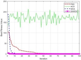
a) Sphere function
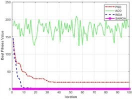
b) Step function
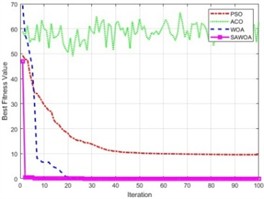
c) Schwefel 2.22 function
To further verify the good performance of the SAWOA, we show the box plots generated by both the SAWOA and WOA, as shown in Fig. 2, as well as the results of the Wilcoxon test analysis and descriptive statistics, as shown in Tables 2-3.
Fig. 2Box plots of the two algorithms
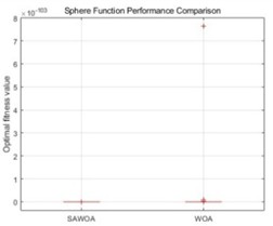
a) Sphere function
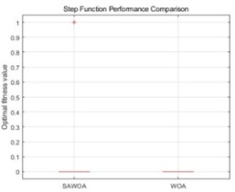
b) Step function
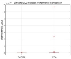
c) Schwefel 2.22 function
Table 2Wilcoxon test results
Sphere | Step | Schwefel2.22 | |
Sample size | 30 | 30 | 30 |
W-statistic | 0 | 0 | 58 |
P value | 0 | 1 | 0.0003 |
Conclude | 0.05 | No significant difference | 0.05 |
Effect size (Cohen’s d) | –0.29 | NaN | –0.33 |
Table 3Descriptive statistics
Algorithm | Sphere | Step | Schwefel2.22 |
SAWOA mean | 2.9415e-117 ± 1.4967e-116 | 0.0000e+00 ± 0.0000e+00 | 3.5718e-68 ± 1.2284e-67 |
WOA mean | 3.3000e-107 ± 1.6247e-106 | 0.0000e+00 ± 0.0000e+00 | 1.0393e-66 ± 4.2740e-66 |
From the above results, the SAWOA algorithm shows excellent optimization performances in most cases, especially in the continuous-type optimization problems. In the sphere function test, the SAWOA achieves amazing optimization results, with the mean value of the optimal solution reaching 2.89×10-1166, which is nearly 20 orders of magnitude greater than the standard WOA’s value of 6.26×10-1055. The p value of the Wilcoxon test is less than 0.001, and the effect size –0.32, which fully proves the effectiveness of the SAWOA improvement strategy; this is mainly because the sinusoidal chaotic initialization can better cover the search space, whereas the adaptive convergence factor effectively balances the contradiction between exploration and exploitation so that the algorithm can quickly and accurately converge to the vicinity of the global optimal solution. The p-value of 0.0003 confirms a statistically significant difference, indicating that SAWOA outperforms WOA under the Schwefel 2.22 benchmark. Although the effect size 0.18 is relatively small, considering that the function contains both linear and nonlinear terms, the SAWOA still maintains a stable optimization performance, which indicates that the algorithm is adaptable to complex problems. Especially when dealing with the product term in the function, the adaptive mechanism of the SAWOA can effectively avoid premature convergence. In the Step function test, although the statistical results show that the difference between the two is not significant (0.25), the SAWOA yields better solutions in some runs. The standard WOA converges to 0 in all but one run, but this may be related to its stronger local search capability.
Thus, the SAWOA significantly improves the optimization performance while maintaining the simplicity of the algorithm through sinusoidal initialization and adaptive convergence factor design. The excellent convergence accuracy and stability of this method make it a new choice for solving complex engineering optimization problems, especially for continuous-type problems. Subsequent studies should focus on enhancing the performance of the algorithm in discrete problems to further expand its application scope.
5.2. Equipment fault identification
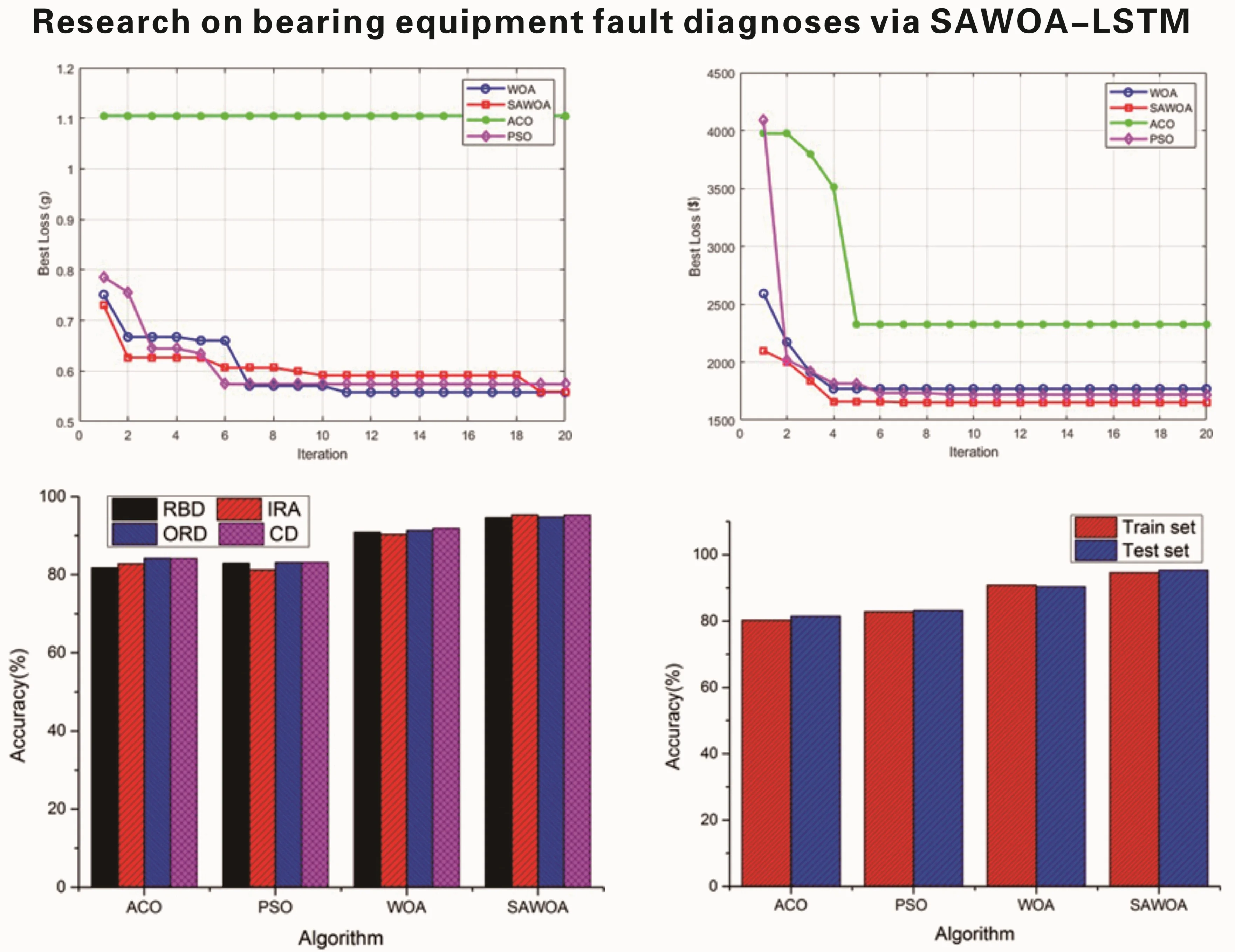
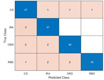
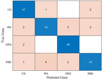
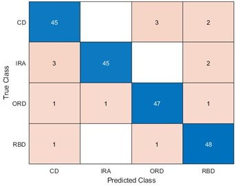
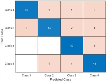
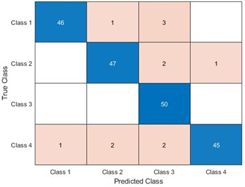
To be able to use LSTM for better identification of equipment faults, optimizing the LSTM model parameters becomes our improvement method. We optimize the number of hidden units and the learning rate of LSTM for four algorithms, namely, ACO, PSO, the WOA, and the SAWOA. The number of hidden units is the key to whether the LSTM network can learn more complex data patterns and features, while an appropriate number of units can improve the generalization ability of the model. The learning rate can improve the model convergence speed and improve the stability of the model, which can enhance the model’s capabilities. Figs. 3-4 show the effects of the LOSS values obtained by using simulated vibration signal data and seasonal sales data as data sources for the four algorithms to optimize the LSTM model under different numbers of iterations. The figure shows that the LSTM model optimized by the SAWOA algorithm proposed in this paper has the smallest BestLoss value in 20 iterations under the same conditions, whereas the SAWOA algorithm always has a lower value, which indicates that the model not only fits well with the training data but also has a better generalization ability, and the number of hidden neurons is obtained as 10 from the 2 plots with a learning rate of 0.001. As shown in Fig. 5, the main part of bearing damage is divided into four types of Rolling Body Damage (RBD), Inner Ring Damage (IRA), Outer Ring Damage (ORD) and Cage Damage (CD). We use the four algorithms to test and verify the prediction performance on the samples of the UI standard dataset-condition monitoring of hydraulic systems. A total of 11935 records were selected, 80 % of which were used in the training set, and 20 % of which were used in the test set. The results of the comparative records are shown in Fig. 6, from which it can be found that the algorithm has better diagnostic results. To further illustrate our recognition effect, we selected 200 bearings from a bearing factory for verification, 50 bearings for each loss type were selected, and the test results obtained via this algorithm are shown in Fig. 5. Fig. 6 shows that this algorithm is able to obtain more accurate identification results in different bearing damage parts; overall, compared with ACO, PSO, and the WOA, the results are improved by 14.17 %, 15.03 %, and 4.32 %, respectively. This finding indicates that optimizing the parameters of the LSTM model via the SAWOA can improve the model performance and detection accuracy. Figures 7-8 show the average effects of the WOA and the SAWOA in the detection of four different types of confusion matrices for different numbers of bearing samples. From the comparison results, the sum of the values of the SAWOA in the main diagonal of the three types of bearings, namely, the RBD, IRA, and ORD, is improved by 1.08 %, 1.62 %, and 1.10 %, respectively, compared with those of the WOA, whereas the values of the CD values are reduced by 0.054 % compared with those of the WOA, so the results of the SAWOA are more stable and have a better detection effect.
Fig. 3Simulated vibration signals
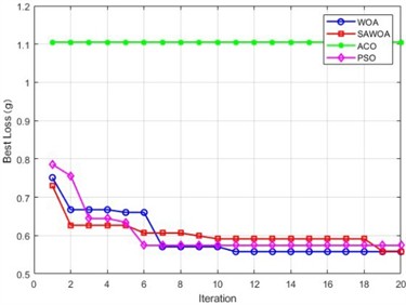
Fig. 4Simulated seasonal sales
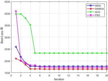
Fig. 5Four types of bearing failures
a) RBD: rolling body damage
b) IRA: inner ring damage
c) ORD: outer ring damage
d) CD: cage damage
Fig. 6Comparison of the prediction accuracies of the four algorithms
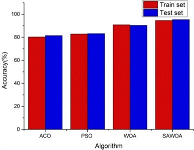
Fig. 7Comparison of the four algorithms for bearing detection
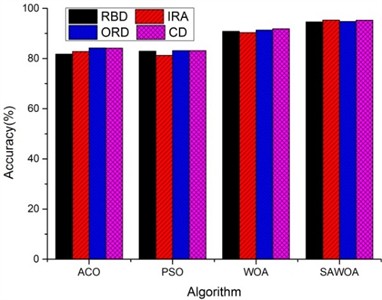
Fig. 8Effectiveness of WOA-LSTM in the diagnosis of four types of bearings
a) RBD detection effect
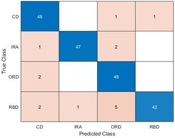
b) IRA detection effect
c) ORD detection effect
d) CD detection effect
Fig. 9Effectiveness of SAWOA-LSTM in the diagnosis of four types of bearings
a) RBD detection effect
b) IRA detection effect
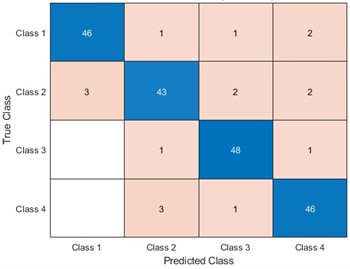
c) ORD detection effect
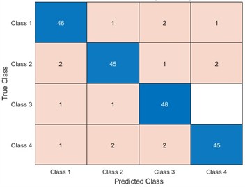
d) CD detection effect
6. Conclusions
To address the shortcomings of the current bearing equipment fault diagnosis methods with low accuracy, in this paper we proposed a strategy for bearing equipment fault diagnoses based on SAWOA-LSTM, and a simulation experiment verified the effectiveness of the method. As a next step, we will further consider the optimization strategy of multiple LSTM parameters to improve the accuracy of the model to identify faults.
References
-
M. P. Sikka, A. Sarkar, and S. Garg, “Artificial intelligence (AI) in textile industry operational modernization,” Research Journal of Textile and Apparel, Vol. 28, No. 1, pp. 67–83, Jan. 2024, https://doi.org/10.1108/rjta-04-2021-0046
-
J. Ma, Y. Xue, Q. Han, X. Li, and C. Yu, “Motor bearing damage induced by bearing current: a review,” Machines, Vol. 10, No. 12, p. 1167, Dec. 2022, https://doi.org/10.3390/machines10121167
-
M. K. Suddle and M. Bashir, “Metaheuristics based long short term memory optimization for sentiment analysis,” Applied Soft Computing, Vol. 131, p. 109794, Dec. 2022, https://doi.org/10.1016/j.asoc.2022.109794
-
S. Mirjalili and A. Lewis, “The whale optimization algorithm,” Advances in Engineering Software, Vol. 95, pp. 51–67, May 2016, https://doi.org/10.1016/j.advengsoft.2016.01.008
-
B. van Hecke, J. Yoon, and D. He, “Low speed bearing fault diagnosis using acoustic emission sensors,” Applied Acoustics, Vol. 105, pp. 35–44, Apr. 2016, https://doi.org/10.1016/j.apacoust.2015.10.028
-
J. M. Guerrero, A. E. Castilla, J. A. S. Fernandez, and C. A. Platero, “Transformer oil diagnosis based on a capacitive sensor frequency response analysis,” IEEE Access, Vol. 9, pp. 7576–7585, Jan. 2021, https://doi.org/10.1109/access.2021.3049192
-
D. Cornel, F. Gutiérrez Guzmán, G. Jacobs, and S. Neumann, “Condition monitoring of roller bearings using acoustic emission,” Wind Energy Science, Vol. 6, No. 2, pp. 367–376, Mar. 2021, https://doi.org/10.5194/wes-6-367-2021
-
C. Yu, Y. Ning, Y. Qin, W. Su, and X. Zhao, “Multi-label fault diagnosis of rolling bearing based on meta-learning,” Neural Computing and Applications, Vol. 33, No. 10, pp. 5393–5407, Sep. 2020, https://doi.org/10.1007/s00521-020-05345-0
-
Q. Fu and H. Wang, “A novel deep learning system with data augmentation for machine fault diagnosis from vibration signals,” Applied Sciences, Vol. 10, No. 17, p. 5765, Aug. 2020, https://doi.org/10.3390/app10175765
-
M. Ge, Y. Lv, and Y. Ma, “Research on multichannel signals fault diagnosis for bearing via generalized non-convex tensor robust principal component analysis and tensor singular value kurtosis,” IEEE Access, Vol. 8, pp. 178425–178449, Jan. 2020, https://doi.org/10.1109/access.2020.3027029
-
Zhu, Q. Gao, D. Sun, and Y. Lu, “A detection method for bearing faults using complex-valued null space pursuit and 1.5-dimensional Teager energy spectrum,” IEEE Sensors Journal, Vol. 20, No. 15, pp. 8445–8454, Aug. 2020, https://doi.org/10.1109/jsen.2020.2983261
-
D. Li, Z. Cai, B. Qin, and L. Deng, “Signal frequency domain analysis and sensor fault diagnosis based on artificial intelligence,” Computer Communications, Vol. 160, pp. 71–80, Jul. 2020, https://doi.org/10.1016/j.comcom.2020.05.034
-
J. Zheng, S. Huang, H. Pan, J. Tong, C. Wang, and Q. Liu, “Adaptive power spectrum Fourier decomposition method with application in fault diagnosis for rolling bearing,” Measurement, Vol. 183, p. 109837, Oct. 2021, https://doi.org/10.1016/j.measurement.2021.109837
-
V. Sharma, N. K. Raghuwanshi, and A. K. Jain, “Sensitive sub-band selection criteria for empirical wavelet transform to detect bearing fault based on vibration signals,” Journal of Vibration Engineering and Technologies, Vol. 9, No. 7, pp. 1603–1617, May 2021, https://doi.org/10.1007/s42417-021-00316-8
-
H. Li, Y. Xu, D. An, L. Zhang, S. Li, and H. Shi, “Application of a flat variational modal decomposition algorithm in fault diagnosis of rolling bearings,” Journal of Low Frequency Noise, Vibration and Active Control, Vol. 39, No. 2, pp. 335–351, May 2019, https://doi.org/10.1177/1461348419846730
-
D. Fernández-Francos, D. Martínez-Rego, O. Fontenla-Romero, and A. Alonso-Betanzos, “Automatic bearing fault diagnosis based on one-class ν-SVM,” Computers and Industrial Engineering, Vol. 64, No. 1, pp. 357–365, Jan. 2013, https://doi.org/10.1016/j.cie.2012.10.013
-
S. S. Roy, S. Dey, and S. Chatterjee, “Autocorrelation aided random forest classifier-based bearing fault detection framework,” IEEE Sensors Journal, Vol. 20, No. 18, pp. 10792–10800, Sep. 2020, https://doi.org/10.1109/jsen.2020.2995109
-
J. Xie, Z. Li, Z. Zhou, and S. Liu, “A novel bearing fault classification method based on XGBoost: the fusion of deep learning-based features and empirical features,” IEEE Transactions on Instrumentation and Measurement, Vol. 70, pp. 1–9, Jan. 2021, https://doi.org/10.1109/tim.2020.3042315
-
L. Eren, T. Ince, and S. Kiranyaz, “A generic intelligent bearing fault diagnosis system using compact adaptive 1D CNN classifier,” Journal of Signal Processing Systems, Vol. 91, No. 2, pp. 179–189, May 2018, https://doi.org/10.1007/s11265-018-1378-3
-
Z. Dong, D. Zhao, and L. Cui, “An intelligent bearing fault diagnosis framework: one-dimensional improved self-attention-enhanced CNN and empirical wavelet transform,” Nonlinear Dynamics, Vol. 112, No. 8, pp. 6439–6459, Mar. 2024, https://doi.org/10.1007/s11071-024-09389-y
-
D. Lee, H. Choo, and J. Jeong, “GCN-based LSTM autoencoder with self-attention for bearing fault diagnosis,” Sensors, Vol. 24, No. 15, p. 4855, Jul. 2024, https://doi.org/10.3390/s24154855
-
F. Althobiani, “A novel framework for robust bearing fault diagnosis: preprocessing, model selection, and performance evaluation,” IEEE Access, Vol. 12, pp. 59018–59036, Jan. 2024, https://doi.org/10.1109/access.2024.3390234
-
K. Han, W. Wang, and J. Guo, “Research on a bearing fault diagnosis method based on a CNN-LSTM-GRU model,” Machines, Vol. 12, No. 12, p. 927, Dec. 2024, https://doi.org/10.3390/machines12120927
-
G. Fu, Q. Wei, and Y. Yang, “Bearing fault diagnosis with parallel CNN and LSTM,” Mathematical Biosciences and Engineering, Vol. 21, No. 2, pp. 2385–2406, Jan. 2024, https://doi.org/10.3934/mbe.2024105
-
W. Liao, L. Wu, S. Xu, and S. Fujimura, “A novel approach for intelligent fault diagnosis in bearing with imbalanced data based on cycle-consistent GAN,” IEEE Transactions on Instrumentation and Measurement, Vol. 73, pp. 1–16, Jan. 2024, https://doi.org/10.1109/tim.2024.3427866
-
Y. Chen, Y. Qiang, J. Chen, and J. Yang, “FMRGAN: feature mapping reconstruction GAN for rolling bearings fault diagnosis under limited data condition,” IEEE Sensors Journal, Vol. 24, No. 15, pp. 25116–25131, Aug. 2024, https://doi.org/10.1109/jsen.2024.3415713
-
S. Hochreiter and J. Schmidhuber, “Long short-term memory,” Neural Computation, Vol. 9, No. 8, pp. 1735–1780, Nov. 1997, https://doi.org/10.1162/neco.1997.9.8.1735
-
B. Alatas, “Chaotic harmony search algorithms,” Applied Mathematics and Computation, Vol. 216, No. 9, pp. 2687–2699, Jul. 2010, https://doi.org/10.1016/j.amc.2010.03.114
-
A. H. Gandomi and X.-S. Yang, “Chaotic bat algorithm,” Journal of Computational Science, Vol. 5, No. 2, pp. 224–232, Mar. 2014, https://doi.org/10.1016/j.jocs.2013.10.002
-
G. Kaur and S. Arora, “Chaotic whale optimization algorithm,” Journal of Computational Design and Engineering, Vol. 5, No. 3, pp. 275–284, Jul. 2018, https://doi.org/10.1016/j.jcde.2017.12.006
-
Y. Li, T. Han, H. Zhao, and H. Gao, “An adaptive whale optimization algorithm using gaussian distribution strategies and its application in heterogeneous UCAVs task allocation,” IEEE Access, Vol. 7, pp. 110138–110158, Jan. 2019, https://doi.org/10.1109/access.2019.2933661
-
D.-G. Kim and J.-Y. Choi, “Optimization of design parameters in LSTM model for predictive maintenance,” Applied Sciences, Vol. 11, No. 14, p. 6450, Jul. 2021, https://doi.org/10.3390/app11146450
-
K. Shirini, M. B. Kordan, and S. S. Gharehveran, “Impact of learning rate and epochs on LSTM model performance: a study of chlorophyll-a concentrations in the Marmara Sea,” The Journal of Supercomputing, Vol. 81, No. 1, pp. 1–18, Dec. 2024, https://doi.org/10.1007/s11227-024-06806-2
About this article

This work was supported by Henan Provincial Science and Technology Research and Development Project (Project Number: 252102210026).
The datasets generated during and/or analyzed during the current study are available from the corresponding author on reasonable request.
The authors declare that they have no conflict of interest.
