Feature extraction and classification of hyperspectral images based on improved two-dimensional compact variational mode decomposition

3.1. Datasets

The data set verified by the experiment is tested and analyzed using two sets of public data sets, which can be obtained [12]. The first Indian Pine Scene data set was collected at the AVIRIS sensor at Indian Pine Proving Ground in northwestern Indiana. The spatial dimension of Indian Pine scene data is 145×145, the spatial resolution is about 20 m, and it is composed of 224 spectral reflection bands. The Indian Anson data space contains two-thirds of agricultural woodland and one-third of forest vegetation.

The available ground features are divided into 16 categories, removing spectral bands containing atmospheric noise and water absorption (bands 104-108, 150-163, 220), reducing the number of original bands to 200. Indian Pine scene data is one of the most commonly used HSIs, and it is also considered a challenging data set. Because the spectral features of some feature classes are very similar, the pixels in the images are heavily mixed. The second dataset of the Pavia University scene was captured by the ROSIS 03 sensor during a flight battle in Pavia, northern Italy. The spatial dimension of the data is 610×340, the spatial resolution is 1.3 m, and the number of spectral bands is 115. After removing 12 noise bands, the remaining 103 bands are processed, and the available ground objects are labeled into 9 categories.

3.2. Metric

There are many indexes to measure the classification Accuracy of different types of ground objects in HSIs, among which the most commonly used indexes include Overall Accuracy (OA), Average Accuracy (AA) and Kappa coefficient [13-15]. The realization of these three indexes is derived from the confusion matrix. The confusion matrix is used to judge whether the classification output is consistent with the real label, as shown below [13]:

In the confusion matrix, diagonal elements represent the number of samples accurately identified for each category, while non-diagonal elements show misjudgments in the classification process, where samples from one category are mistakenly assigned to another. Through the confusion matrix, the number of correct classification and misclassification of each type can be visually observed. However, it is not intuitive to judge the classification effect directly from the confusion matrix, so a variety of indexes to measure the classification accuracy have been derived, such as overall accuracy (OA), average accuracy (AA) and Kappa coefficient, etc. These indexes are widely used to evaluate the classification performance. Where, $c_{ii}$ represents the number of class $i$ samples that are correctly classified, $c_{ij}$ represents the number of class $i$ samples that are classified to class $j$, and $r$ is the total number of categories of samples. The overall classification accuracy refers to the percentage of the number of correctly classified pixels in the entire image. Through this index, the quality of the classification results can be intuitively seen. The definition is as follows [9]:

Although the overall classification accuracy can effectively reflect the overall accuracy of classification results, it shows certain limitations in the face of multi-class cases where the number of samples varies greatly between classes. Specifically, its assessment results may be dominated by those categories with large sample sizes, which may not accurately reflect the classification performance of all categories. The average accuracy, the arithmetic average of the accuracy of each category, provides a way to evaluate the impact of different categories on the overall classification effect, and more comprehensively measures the performance of the classifier on each category. Its definition is as follows [9]:

where $c_{ii}$ represents the number of class $i$ samples that are correctly classified, $c_{+i}$ represents the pixel number classified into class $i$ at the time of prediction.

The Kappa coefficient fully considers the impact of uncertainty on classification results, is used to test the degree of consistency, and can objectively measure the overall result of classification. Its definition is as follows [9]:

where, $N$ represents the total number of samples, $c_{i+}$ represents the real pixel number of class $i$, and $c_{+i}$ represents the pixel number classified into class $i$ at the time of prediction.

For the classification effects of different HSI ground object categories, we conducted a comparative analysis using the measurement indicators OA, AA and Kappa. OA represents the total accuracy rate of classification. Referring to Eq. (6), the larger the OA value, the better the overall classification effect of the ground object category. AA is a classification measurement index for each type of ground object. Referring to Eq. (7), the larger the AA value, the better the classification effect of a certain type of ground object. Referring to Eq. (8), the Kappa coefficient is a ratio that represents the reduction in errors between a classification and a completely random classification.

3.3. Experimental flow chart

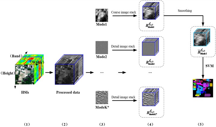
The flow chart of the experimental simulation is shown in Fig. 1. The 2D-C-VMD of each band of the original HSI is carried out separately. The 2D-C-VMD can decompose each 2D band image of HSI into sub-band images of different scales. It is worth noting that the number of sub-band images obtained by decomposition is what we first need to give, that is, the prior parameter $K$ value. In literature [16], we explained the prior parameter $K$ value in detail. The sub-band images of different scales obtained from each 2D image decomposition are stacked respectively, and several feature samples of different scales are obtained. Also known as in Fig. 1 is first decomposed Mode 1, Mode 2 and Mode K respectively to carry on the stack, respectively get $B_{Mode1}^{f_{(i,j)}^l}$, $B_{Mode2}^{f_{(i,j)}^l}$ and $B_{ModeK}^{f_{(i,j)}^l}$. The $f_{(i,j)}^l$ is used to represent each 2D band image of the HSI, $l$ represents the number of bands, and $(i,j)$ represents the spatial position of each band. Then, the first mode component obtained by decomposition is smoothed again to obtain the smoothed feature information sample. Finally, the feature information sample is classified by support vector machine and compared according to the analysis result.

Below we give a detailed description of the flow chart in Fig. 1.

Step 1: Two original data sets, Indian Pine and Pavia U, were selected to remove the band images with heavy noise pollution. HSI data is expressed as $R^{\{W\times H\times L\}}$, $W$ represents the width of spatial dimensional data, $H$ represents the height of spatial dimensional data, and $L$ represents the total number of bands of HSI.

Step 2: Each spatial image ($f_{(i,j)}^l$) is decomposed by 2D-C-VMD, and several mode components are obtained respectively, and then each mode component is re-stacked, respectively get $B_{Mode1}^{f_{(i,j)}^l}$, $B_{Mode2}^{f_{(i,j)}^l}$ and $B_{ModeK}^{f_{(i,j)}^l}$.

Step 3: Repeat step 2 to decompose the decomposed $B_{Mode1}^{f_{(i,j)}^l}$ again by 2D-C-VMD, and stack the first pattern component obtained by decomposition, then get respectively ${\stackrel{-}{B}}_{Mode1}^{f_{(i,j)}^l}$.

Step 4: The SVM classification and effect analysis were carried out on the pattern component features obtained from the third step decomposition.

It is worth noting that the influence of the prior parameter $K$ value should be considered when performing the 2D-C-VMD decomposition in step 3. Here, we refer to the scheme proposed in reference [16] for the optimal $K$-value screening process.

Fig. 1Feature extraction and classification of HSIs with improved 2D-C-VMD

3.4. Analysis of experimental results

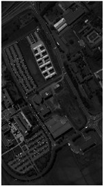
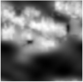
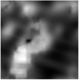
In Fig. 2, sub-band images of Indian Pine and Pavia University at 4 different scales were obtained by 2D-C-VMD in the 23rd band and the 30th band, respectively. In the literature [16], we discussed and analyzed the prior parameter K values of different HSIs. The original 23th-band and 30th-band images of the two data sets are shown in subgraphs a) and b) of Fig. 2. From the decomposed sub-band images of different scales, we can clearly see that the first sub-band obtained from the decomposition of the two sets of data contains the low-frequency contour component feature information in the original image. Subsequent sub-band images contain high frequency detail feature information of edges and textures in the original image.

According to the preliminary classification results of different features, the results of the first mode component of the two sets of data are the best. It shows that the first low-frequency mode component obtained by decomposition can suppress the adverse effect of spatial domain noise on classification. At the same time, we also compare and analyze the feature information of different scale sub-band images. In order to further mine the effective feature information of the first mode component obtained by decomposition, we perform the two-dimensional compact variational mode decomposition on the first mode decomposition again to extract more effective feature information conducive to classification.

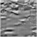
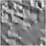
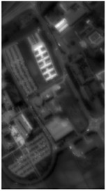
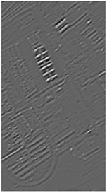
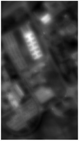
In Fig. 3, we again use 2D-C-VMD for the first optimal mode component from the Indian Pine and Pavia University decomposition. Through comparative analysis of several experiments, we took 3 and 4 prior parameters of the data sets of Indian Pine and Pavia university respectively. From the decomposition of the 23 band and 30 band in Fig. 3 to obtain sub-band images of different scales, we can find that the first mode component obtained by decomposition is smoother.

Fig. 2Sub-band images of different scales obtained by 2D-C-VMD decomposition of Indian Pine and Paiva University

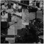
a) IP Band 23

a1) Mode 1

a2) Mode 2

a3) Mode 3

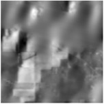
a4) Mode 4

b) PU Band 30

b1) Mode 1

b2) Mode 2

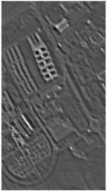
b3) Mode 3

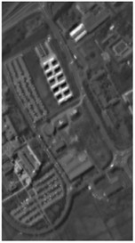
b4) Mode 4

Fig. 3Sub-band images of different scales obtained by 2D-C-VMD of the optimal low-frequency component

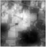
a) Original IP image

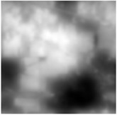
a1) Mode 1

a2) Mode 2

a3) Mode 3

b) Original PU image

b1) Mode 1

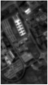
b2) Mode 2

b3) Mode 3

b4) Mode4

Table 2 and Table 3 show the classification of Indian Pine and Pavia University data sets under different schemes. The measurement indexes were represented by AA, OA and Kappa respectively. Select 10 % and 2 % of different feature information as the training set, and the rest as the test set. We choose the support vector machine network with good classification performance for small sample data, and the network adopts cross-validation for parameter optimization. The Raw in Table 2 and Table 3 represent the results of support vector machine classification directly on the original data set. L-2D-C-VMD means that the optimal low-frequency component obtained from the first decomposition is decomposed again by two-dimensional compact variational modes. Let's focus first on the OA metric, because from this metric we can see the overall performance of a category in the data set. It can be seen from the classification effect that the OA value of the original Indian Pine was 78.70 % directly identified by classification, and after the first 2D-C-VMD decomposition, the OA value was increased to 97.57 %.

After the first filtering, the classification performance of different feature categories is greatly improved. However, after we smoothed the optimal low-frequency component again, there was also a small increase in the value of OA in the dataset Indian Pine. In the OA index, the overall OA decreases due to the influence of category 9. In the dataset Pavia university, the OA value of the original Raw was 87.03 %, and after the first 2D-C-VMD processing, the OA value became 95.21 %, which suppressed the adverse impact of spatial dimension noise on classification to a certain extent. Similarly, after smoothing and filtering the first mode component, OA value increased by about 1.7 %, Kappa increased by about 2 %, and AA increased by about 3 %.

In order to avoid the contingency of the results of a single training sample, we selected different proportions of training samples from Indian Pine and Pavia University as the training set, and the rest as the test set for comprehensive comparative analysis. Here, OA and Kappa indexes are selected for metric analysis. Support vector machine classifier is also used to evaluate the classification of ground objects under different training samples. In Fig. 4, the OA and Kappa values of the recognition results of Indian Pine training samples at 4 %, 7 %, 10 % and 20 % are given. From the OA and Kappa values, it is obvious that after 2D-C-VMD spatial filtering, the classification performance of support vector machine network can be further improved while overcoming spatial noise interference. In Fig. 5, the OA and Kappa values of Pavia University training samples under 0.5 %, 1 %, 2 % and 5 % are given.

By combining the recognition effect of Fig. 4 and Fig. 5, we can conclude that the classification performance of different ground objects can be further improved after the quadratic 2D-C-VMD of the original HSI, and the adverse effects of spatial domain noise on classification can be suppressed to a certain extent. At the same time, in the case of less training samples, the recognition effect advantage is more obvious through the secondary use of 2D-C-VMD.

Fig. 4Classification of OA and Kappa values of Indian Pine data under different training samples

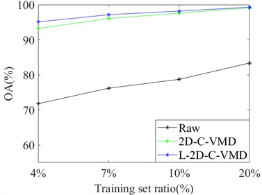
a) OA

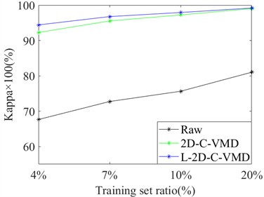
b) Kappa×100

Fig. 5Classification of OA and Kappa values of Pavia University data under different training samples

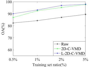
a) OA

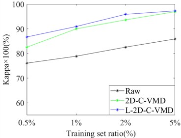
b) Kappa×100

In Table 4, we make a comparative analysis of different spatial domain methods. Indian Pine and Pavia University datasets selected 10 % and 2 % training samples respectively as training sets, and the rest were used as test sets. The classifier still uses the support vector machine as the classifier.

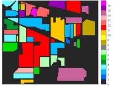
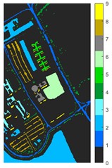
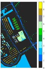
Fig. 6 and Fig. 7 respectively show the color maps of different feature classification effects of Indian Pine and Pavia University data sets under different spatial domain feature extraction methods. Subfigure a) is the color map label for the different features of the original data set. Raw represents a rendering of the original data set directly classified by support vector machine. The closer the classification color image effect is to subfigure a), the better the feature extraction effect is. From Fig. 6, you can see that there are between 1 and 16 different color labels, and each color represents a feature category. The details of each feature category can be combined with the list given in Table 1. It can be seen from the color map of classification that the feature information extracted by 2D-EWT in Indian Pine data is less effective than 2D-EMD and 2D-C-VMD. The effect of 2D-EMD is close to that of 2D-C-VMD. After using 2D-C-VMD twice, the classification effect is improved to some extent. Improved from the original OA value of 78.7 % to 98.17 %. There are a total of 9 ground object categories in the data of Pavia University, and the reference value OA given is 87.03 %. After the extraction of spatial domain features, the classification effect has been improved to a certain extent.

Fig. 6Classification results of Indian Pine dataset under different spatial domain methods

a) Classified color chart

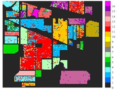
b) Raw

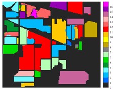
c) 2D-EMD

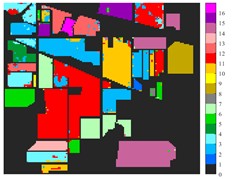
d) 2D-LP-EMD

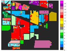
e) 2D-T-EMD

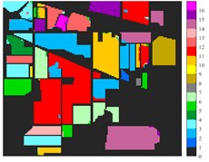
f) 2D-C-VMD

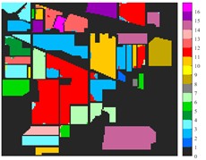
g) L-2D-C-VMD

From the classification effect, 2D-C-VMD spatial domain filter has the best OA value enhancement effect. When 2D-C-VMD is used again to filter the optimal low-frequency component obtained from the first decomposition, it can be seen from the OA and Kappa indexes that there is also some room for improvement. In addition, after the previous discussion of different spatial domain methods, 2D-EMD uses iterative decomposition to obtain several inherent mode components, and the algorithm convergence speed is slow and the computational efficiency is low, so it often requires more computational costs when processing HSIs containing multiple bands. 2D-EMD also lacks theoretical support in mathematical theory. There are many sub-methods of 2D-EWT, so 2D-LP-EWT and 2D-T-EWT are selected here for comparative analysis. The 2D-EWT combines the adaptability of EMD and the theoretical completeness of wavelet, and can be used for feature extraction of hyperspectral images. From the classification effect of feature extraction, there is still a large room for improvement. Using the variational idea in mathematics, the 2D-C-VMD method can decompose the original image into sub-band images of different scales. The variational idea can screen several sub-band images of different scales at the same time. The decomposition of each sub-band image has a good timeliness, which can greatly save the time of feature extraction. In literature [16], we carried out relevant research and analysis.

According to the classification performance of Indian Pine and Pavia University data sets under different spatial domain methods, the smooth classification effect of 2D-C-VMD in the two sets of data is better. The method is simple and easy to operate. It smoothed the first mode component obtained by decomposition. According to the classification effect, 2D-C-VMD has good robustness in smoothness.

Fig. 7Classification results of Pavia University dataset under different spatial domain methods

a) Classified color chart

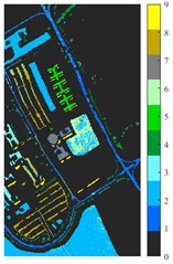
b) Raw

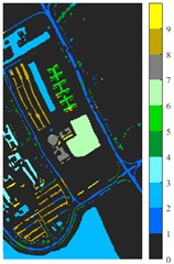
c) 2D-EMD

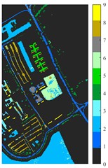
d) 2D-LP-EMD

e) 2D-T-EMD

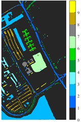
f) 2D-C-VMD

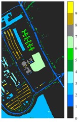
g) L-2D-C-VMD