Research on converter transformer state early warning system based on confidence ratio-EEMD and multi-cascade network

1. Introduction

As the core equipment of the power system, the operation status of the converter transformer directly determines the operation safety, stability and power supply reliability of the entire power system. In terms of equipment safeguard measures, in addition to the intelligent analysis of operation early warning data, innovative methods such as dynamic characteristics research based on thermodynamic simulation models and intelligent operation and maintenance strategies based on condition assessment have shown remarkable results. Typical applications, such as the dynamic thermal assessment model and preventive intelligent operation and maintenance scheme proposed in a literature, effectively improve the operation efficiency and life cycle management level of equipment by establishing a multi-physics coupling simulation system and an adaptive maintenance cycle algorithm [1]. The finite element simulation method was used to numerically simulate the ambient airflow distribution and the oil flow and temperature distribution of the converter transformer with or without Box-in structure, and the influence of the existence of Box-in structure on the temperature rise of the converter transformer was analyzed, and the ventilation strategy of the Box-in structure converter transformer was studied. The multi-dimensional parameter analysis and predictive early-warning technology for converter transformers fundamentally involve the systematic investigation of dynamic operational characteristics, including but not limited to electromagnetic field distributions, partial discharge acoustic emission signatures, fiber-optic temperature field gradients, multi-physics coupling thermodynamics, and dissolved gas chromatography profiles in insulating oil. Through the integration of high-fidelity data acquisition systems with advanced analytics frameworks (e.g., machine learning-driven multi-parameter fusion algorithms and deep neural network-based pattern recognition), this holistic approach enables comprehensive operational diagnostics and intelligent anomaly prediction. The methodology aims to achieve threefold objectives: early detection of incipient insulation degradation, proactive fault mitigation through adaptive threshold optimization, and ultimately enhancing operational reliability while optimizing maintenance strategies and extending critical equipment service lifespan. When the equipment is running normally, the partial least squares regression (PLS) method is used to mine the correlation between state parameters and the regression equation, and a principal component analysis based on the deviation between the regression prediction and the actual is constructed [2]. (PCA) commutation state evaluation method. Currently, there are many methods for monitoring the operating status of converter transformers. Assessing the earth current of the steel core can directly indicate the grounding fault of the steel core [2, 3]. According to the characteristics of abnormal values in oil chromatography monitoring data, a variety of multi-element detection methods have been proposed to more clearly reflect the changes in the operating status of the equipment through the tracking and evaluation of the abnormal value intervals; and temperature data is also a very important source of evaluation information for converter transformers [4, 5]. Establish the thermal circuit model of the converter transformer through thermoelectric analogy or gray correlation analysis method, and set the load and status evaluation model based on the temperature rise characteristics [6]. Current status warnings for converter transformers and other equipment often consider the possible fluctuations or trend changes in the internal parameters of the converter transformer in the future period and issue early warning information to ensure that risk losses are within a tolerable range. Literature [7] realizes effective feature extraction of equipment operating status data through unsupervised training of deep belief networks, and then constructs a health index of equipment operating status to provide early warning of its status. At present, most parameter sequence prediction and warning are grounded in numerical statistical models, such as ARIMA [8], ARIMAX [9], VAR [10] and GARCH [11], etc. Nevertheless, as many of these frameworks are grounded in established numerical equations, they are insufficient to comprehensively capture the attributes of the temporal sequence. In addition, nearly all converter variable parameter sequences are complex and variable, so it is challenging to achieve optimal forecast outcomes. By considering parameter sequence prediction as a feature analysis issue with dynamic parameters, although deep learning methods perform well on simple data sets, it remains challenging to capture the complex nonlinearity across various factors on non-stationary commutation time series data [12]. relationship, resulting in poor early warning effect.

At the same time, because the existing state analysis and monitoring use a single level of information source, the parameter data processed are often non-stationary and incomplete, making it difficult to ensure the reliability and comprehensiveness of the converter transformer state warning and the accuracy of the converter transformer. Accuracy of risk assessment. Therefore, the current focus of research is on multi-source information fusion. Multi-source parameter sequence fusion is to comprehensively consider different information sources in space and time to extract the nonlinear and unstable characteristics of its internal whole, and obtain a consistent representation or description through the auxiliary fusion of parameters, so that it can the accuracy of the evaluation results is guaranteed [13]. In Ref. [14] first calculated the temperature field and moisture distribution, and then established a dynamic deduction model of the degree of aggregation distribution with improved moisture translation factor. Finally, the Delaunay triangulation model was used to evaluate the distribution of insulation aging state parameters in the equipment. Ref. [15] relying on tensor combination, the characteristic merging of wear indicators such as temperature, voltage and current is constructed, and a comprehensive degradation evaluation index of the converter transformer winding is constructed to achieve early warning of insulation degradation status. In terms of alarm information, the current alarm basis in the converter station only comes from the safety thresholds and deviations of power equipment in the safety instructions or simple modeling characteristics of the signals sent by the equipment, which lacks intelligence and is not enough to cope with different characteristics. Various types of faults [16].

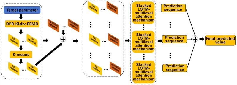
Aiming at the two problems of poor prediction results of equipment non-stationary parameters and improving the diversity and flexibility of early warning results. This paper proposes a converter transformer state early warning system with DPR-KLdiv-EEMD and multi-cascade network. First, the commutation variable parameter sequence is decomposed into multiple subsequences through the ensemble empirical mode decomposition method (EEMD), and the DPR-KLdiv confidence ratio is used to eliminate false decomposition components to enhance robustness. Then, the adaptive clustering algorithm is used to perform analysis on the subsequences. Clustering and reconstruction to decrease the complexity and computational time of parameter forecasting. Then multi-level subsequences and other equipment parameter sequences are used as multi-dimensional inputs of the multi-cascade network for subsequence prediction. The predicted values of each subsequence are finally added to achieve the ultimate predicted value of the objective parameter sequence. Multi-cascade networks can successfully identify the interdependencies between multiple factors and the chronological characteristics of multi-variable time series by stacking residual units and LSTM subnets. While introducing the generalization characteristics of parameters, uses fuzzy set thinking to improve the single problem of early warning results in expert rules and improve the robustness of the early warning system.

2. Multivariate forecast

During normal operation of the converter transformer in a converter station, its insulation system inevitably ages or deteriorates under stresses from electrical, thermal, mechanical, and other physical forces. This results in material degradation, cracking, and decomposition, leading to the production of certain low-molecular-weight hydrocarbon gases such as hydrogen, which dissolve in the oil. Concurrently, parameters like oil temperature, winding temperature, operating current, and voltage may exhibit fluctuations or trends over time. Timely identification of these parameter trends is crucial for accurate health assessment and abnormal condition alerts of the equipment status.

Monitoring these critical parameters can facilitate more precise evaluations of the equipment's health condition, providing a scientific basis for preventive maintenance and ensuring the safe and stable operation of power systems. Effective monitoring not only aids in detecting potential issues but also guides maintenance personnel in taking appropriate actions to prevent failures, thereby enhancing the reliability and efficiency of the power grid.

2.2. DPR-KLdiv-EEMD decomposition and clustering

Literature [17] highlights the necessity and nonlinearity of considering sparse characteristics and local features in image reconstruction. For the prediction of electrical parameters, the problem can be framed as a multi-level sequence reconstruction task, where the sparsity and locality of these parameters must also be taken into account.

Incorporating sparse characteristics and local features is essential for accurately capturing the intrinsic properties of the data, which enhances the precision of image reconstruction and electrical parameter prediction. By addressing the multi-level nature of these tasks, models can better represent complex relationships within the data, leading to improved performance and reliability. This approach ensures that both global structures and fine details are preserved, providing a more robust solution for applications requiring high accuracy and detailed analysis. EEMD (Ensemble Empirical Mode Decomposition) is a data-driven, adaptive algorithm designed for the analysis of nonlinear and non-stationary signals. This method effectively decomposes complex signals into simpler intrinsic mode functions (IMFs), enabling detailed examination of various frequency components within the signal. By adaptively adjusting to the characteristics of the data, EEMD overcomes many limitations of traditional signal processing techniques, making it particularly suitable for analyzing signals with time-varying frequencies and amplitudes. Its ability to handle nonlinearity and non-stationarity makes EEMD a powerful tool for applications ranging from biomedical signal processing to environmental data analysis, proposed by Wu and Huang [18]. By introducing ensemble empirical mode decomposition (EEMD), the complex target sequence is broken down into M simpler subsequences, with each subsequence representing the characteristics of the original parameter sequence at different time scales. This decomposition allows the subsequent prediction process to focus specifically on capturing and analyzing the inherent patterns within each corresponding time scale. By concentrating on these individual time-scale-specific behaviors, the approach enhances the accuracy and robustness of the component predictions. This method ensures that the unique dynamics at various time scales are properly accounted for, leading to more reliable and precise forecasting outcomes.

Assuming that the original parameter sequence is $X=\left\{x_1,x_2,\dots ,x_T\right\}\in R^T$, $X$ is decomposed through EEMD, and then $M-1$ IMF components and a residual component $r$ are obtained:

3

$X={\sum }_{j=1}^{M-1}{c}^j+r.$

Among them, $j=1...M-1$, by iterating $I$ rounds of decomposition and calculating the average value of IMF and $r$, the final decomposition result is obtained:

4

$IM{F}^j=\frac{1}{I}{\sum }_{i=1}^I{c}^{i,j},\left(j=1,...,M-1\right),$

5

$R=\frac{1}{I}{\sum }_{i=1}^l{r}^i.$

Finally simplified to:

6

$S=\left\{s^1,s^2,...,s^M\right\}\in {\mathbb{R}}^{M\times T}.$

Due to the frequency tail effect [19] during the decomposition process, False IMF components can be generated during the decomposition process, necessitating a filtering step to select the parameter subsequences that most accurately reflect the operating parameters of the converter transformer. This selection is crucial for ensuring the convergence of connected inputs in subsequent multi-level analyses.

To address this, an IMF selection method based on the proportion of Dynamic Parameter Ratio (DPR) to Kullback-Leibler divergence (KLdiv) is introduced. Additionally, adaptive thresholding techniques are employed to identify the most meaningful IMFs that are closely related to the parameters essential for early warning systems in converter transformers [20].

This approach ensures that only the most relevant and informative IMFs are used in further analysis, enhancing the accuracy and reliability of the predictions. By focusing on these significant components, the system can better capture the underlying dynamics of the transformer’s operational parameters, leading to improved performance and more effective early warnings. DPR has the capability of identifying the emergence and strength of particular parameter sequence frequency components and their multiples in the extracted envelope power spectrum. Therefore, DPR can be used to quantify subsequences dependent on the quantity of useful data in a specific IMF. Since particular frequency components are associated with warning categories, harmonic frequencies matching to $1/3X$, $1/2X$, $2/3X$, $1X$, $4/3X$, $3/2X$ and $5/2X$ were chosen (where 1$X$ represents the key oscillation). $DPR$is calculated based on the ratio between the parameter-specific frequency component corresponding to the warning category and the irrelevant residual frequency component [21, 22]:

7

$DPR\left(n\right)=10\times \mathrm{l}\mathrm{o}\mathrm{g}\left(\left\{\frac{{\sum }_{j=1}^{N_{wfr}}FF{C}_n^2\left(j\right)}{{\sum }_{j=1}^{N_{\eta fr}}RF{C}_n^2\left(j\right)}\right\}+10\right),n=\mathrm{1,2},3,\dots ,IM{F}_n.$

In this context, $n$ represents the number of IMF components, ranging from 1 to 10, and $j$ is the index of the subsequence frequency. The index $j$ denotes a specific frequency range within the broader frequency range of interest, which corresponds to the narrowband frequency range relevant to the early warning classification parameters.

To elaborate, each value of $j$ identifies a particular narrowband frequency range that is significant for the analysis. These ranges are critical because they help pinpoint specific frequency points associated with the early warning parameters. By focusing on these precise frequency ranges, the method ensures that the most pertinent frequency components are analyzed, enhancing the accuracy of the early warning system for the converter transformer. This targeted approach allows for more effective monitoring and detection of potential issues by concentrating on the frequencies where meaningful changes are likely to occur. FFC denotes the energy of the $j$-th frequency component near the $n$-th order IMF component, representing the energy associated with a specific frequency that is relevant to commutation change warnings. RFC, on the other hand, represents the remaining frequency components within the same frequency range that are not related to early warning signals. These RFC components reflect the energy of parameter components that are not pertinent to the warning signals. $N_{wfr}$ is the number of frequencies surrounding a specific frequency component. represents the overall count of frequencies within the limited spectral band. And $KLdiv$ calculates among the likelihood distribution function (PDF) from the derived subsequence and the parameter sequence:

8

$KLdi{v}_n={\sum }_{z\in Z}PDF\left(z\left(t\right)\right)ln\left(\frac{PDF\left(z\left(t\right)\right)}{PDF\left(IM{F}_n\left(t\right)\right)}\right).$

Among them, $PDF\left(IMFn\left(t\right)\right)$ is the probability amplitude of the $n$-th extracted IMF, and $PDF\left(z\left(t\right)\right)$ is the PDF of the converter variable parameter sequence $\left(z\left(t\right)\right)$. The value of $KLdiv$ varies between 0 and 1, where a value adjacent to nothing indicates that the PDF of the $k$-th IMF and the PDF of the parameter sequence are close to each other, that is, the IMF and the parameter sequence are similar in probability distribution and may contain more relevant and useful information.

For this purpose, the final target ratio of the IMF is:

9

$Ob{j}_n=\frac{DP{R}_n}{KLdi{v}_n}.$

Finally, significant IMF components are selected by comparing the indicator ratios derived from the subseries against predefined thresholds. IMFs that fall below the threshold are excluded and do not participate in subsequent clustering operations.

Furthermore, this paper uses an adaptive threshold method to choose significant IMF elements. Inspired by the concept of “universal threshold” widely used in the field of signal search [23], this paper proposes the following formula to calculate the adaptive threshold for IMF selection:

10

$adTh=var\sqrt{2\mathrm{l}\mathrm{o}\mathrm{g}N}.$

Among them, var is the variance of the normalized ratio, and $N$ is the total number of IMFs.

Fig. 1 illustrates a sample of breakdown by raw EEMD on a sequence of oil temperature data length 1024.

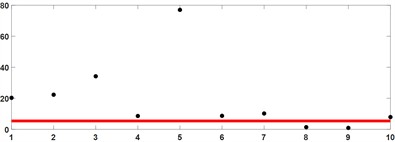
Calculate the ratio of DPR and $KLdiv$, which is the ratio of each IMF component to the original parameter sequence. The results are shown in Table 1. It can be seen that the 9th and 10th components have lower ratios than other IMF components as shown in Fig. 1, and are filtered through adaptive thresholds as shown in Fig. 2. From a similarity perspective, they can be regarded as false IMF components and do not participate in subsequent operations.

Table 1DPR-KLdiv-IMF component similarity

IMF	5	3	2	1	7	6	10	4	8	9
Objk	77.0	34.2	22.2	20.3	10.2	8.7	7.9	8.6	1.4	0.9

Fig. 1EEMD decomposition results of oil temperature data

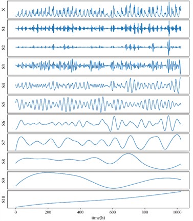
Visible is that the initial intricate parameter sequence is simplified following decomposition into 10 subsequences (9 IMFs and 1 residual). Nevertheless, if each subsequence is modeled directly, the overall computational time will increase significantly. Therefore, it is required to minimize the quantity of subsequences and enhance forecast accuracy through clustering and reconstruction.

Fig. 2IMF optimization selection

For clustering indicators, K-means clustering [23] is a commonly used data mining technique used to divide a dataset into k different clusters, where the data of each cluster has a high similarity. This algorithm is a type of partitioned clustering method whose goal is to minimize the sum of squares within a cluster (i.e., the sum of squares of the distance between a point in a cluster and the center of a cluster). The following are the basic principles and steps of K-means clustering.

The K-means algorithm operates on the principle of minimizing intra-cluster variance. Intra-cluster variance is the sum of squares of the distance from a point in a cluster to the centroid of the cluster. The algorithm tries to find a way to allocate the total intra-cluster variance to the minimum.

1.Select the initial centroid: First, $k$ points are randomly selected from the dataset as the initial centroid. 2. Assign data points to the nearest centroid: For each data point in the dataset, assign it to the cluster corresponding to the nearest centroid based on some distance metric (usually Euclidean distance). 3. Update Centroid Position: For each cluster, recalculate its centroid. The new centroid is the average of the points in the current cluster. 4. Repeat steps 2 and 3: Repeat the process of data point assignment and centroid update until a certain stop condition is met. A stop condition can be that the centroid no longer changes significantly, that a predetermined maximum number of iterations is reached, or that the variation in the intra-cluster variance is less than a certain threshold.

This article uses sample entropy (SE) to assess the complexity of every subsequence [24]. The greater sampling complexity, the greater the intricacy in the sequence, and the amount of information contained in the subsequences approximated by the sample entropy is similar.

The sample entropy for a parameter sequence $X=\{x_1,x_2,...,x_T\}\in R^T$ is defined as follows.

(1) Convert the parameter sequence into a set of $M-1$ dimensional vectors:

11

$X^i=\left\{x_i,x_{i+1},...,x_{i+m-1}\right\}\in {\mathbb{R}}^T,\left(i=1,...,T-m+1\right).$

(2) Define $d$ as utmost difference in the number of related sequences between $X^i$, $X^j$:

12

$d\left(X^i,X^j\right)=\mathrm{m}\mathrm{a}\mathrm{x}{}_{k=0,...,m-1}\left(\left|x_{i+k}-x_{j+k}\right|\right).$

(3) Calculate the overall count of $<r$ for each $i$ value $B_i^m$ and the mean $B^m$:

13

$B_i^m=\frac{1}{T-m+1}num{}_{j\ne i},\left\{d\left(X^i,X^j\right)<r\right\},$

14

$B^m=\frac{1}{T-m}{\sum }_{i=1}^{T-m}{B}_i^m.$

(4) Finally, the sample entropy of each subsequence is calculated:

15

$SE\left(m,r,X\right)=-{\ln B}^m,$

16

$E=\left\{e_1,e_2,...,e_M\right\}\in {\mathbb{R}}^M,$

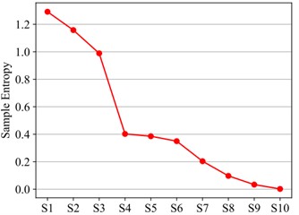
where $e_i=SE\left(m,r,s^i\right)\text{,}$$(1\le i\le M)$ represents the sampling complexity of the $i$-th subsequence. Fig. 3 indicates the sampling complexity of every subsequence in Fig. 1. Notice that its value diminishes as the frequency of the subsequence decreases from high toward low, and the intricacy also lessens.

Fig. 3Subsequence sample entropy

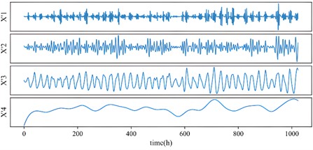
Then, this paper adaptively clusters the subsequences into $K$ groups based on the value of sampling complexity through the K-means method [24] as shown in Fig. 4. This article sets $K=\text{4}$; Table 1 displays the results achieved by using K-means to the subsequence depicted in Fig. 1 when $K=\text{4}$.

Table 2Clustering results of K=4

Clustering	C1	C2	C3	C4
Subsequence	S1, S2	S3	S4, S5, S6	S7, S8

By accumulating the subsequences within each group derived by K-means, the associated novel subsequence can be rebuilt:

17

$X^{\text{'}i}={\sum }_{s\in C_i}s,\left(i=\mathrm{1,2},...,K\right).$

The new subsequence obtained following reconstruction based on the results shown in Table 2 is depicted in Fig. 3.

Fig. 4New subsequence of K= 4

2.3. Converter parameter prediction model

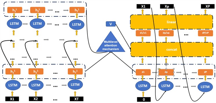
The prediction module of this system builds a prediction model based on multi-cascade connections to completely extract characteristics from multi-variable temporal sequences and create predictions. As shown in Fig. 5, The framework is grounded on the encoding-decoding structure, by layering residual-LSTM as the input processor and a single-layer LSTM as the output generator [25]. During forecasting, the input processor extracts characteristics from the input multidimensional temporal sequences with a temporal window of length $T$ and compresses them into a context vector of a constant size. Next, the output generator progressively translates the data in the context vector to achieve the forecasted value of the upcoming period $p$.

Fig. 5Multi-cascade prediction network

2.3.1. Encoder

To extract temporal characteristics from multi-parameter sequences, this article uses LSTM as the fundamental component of the input processor. LSTM, or Long Short-Term Memory, is an advanced variant of Recurrent Neural Networks (RNN) renowned for its superior capability in modeling sequential data. While it operates similarly to traditional RNNs by updating its hidden states based on current inputs to encapsulate both short-term and long-term dependencies within sequences, LSTM introduces a distinctive feature: a gating mechanism. This allows the LSTM to selectively maintain or forget historical information, effectively addressing the common problems of vanishing or exploding gradients encountered in conventional RNNs when processing extended temporal sequences. As depicted in the Fig. 6, an LSTM cell comprises a memory state $C_t$ alongside three gates: the forget gate, the input gate, and the output gate. These components work together to regulate the flow of information into and out of the memory state, enhancing the model's ability to manage complex sequences efficiently.

Fig. 6LSTM network structure

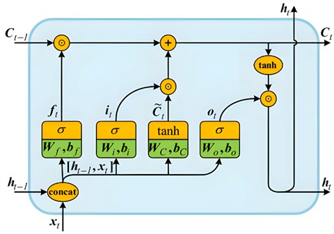
As shown in Fig. 6, the revision process of the LSTM cell with internal layer dimension $H$ is:

18

$\left\{\begin{array}{l}{f}_t=\sigma \left(W_f\cdot \left[h_{t-1},x_t\right]+b_f\right),\\ i_t=\sigma \left(W_i\cdot \left[h_{t-1},x_t\right]+b_i\right),\\ o_t=\sigma \left(W_o\cdot \left[h_{t-1},x_t\right]+b_o\right),\\ {\tilde{C}}_t=\mathrm{t}\mathrm{a}\mathrm{n}\mathrm{h}\left(W_C\cdot \left[h_{t-1},x_t\right]+b_C\right),\\ C_t=C_{t-1}\odot f_t+{\tilde{C}}_t\odot i_t,\\ h_t=\mathrm{t}\mathrm{a}\mathrm{n}\mathrm{h}\left(C_t\odot o_t\right),\end{array}\right.$

where $[h_{t-1},x_t]\in {\mathbb{R}}^{H+N}$ is the connection between the prior hidden condition $h_{t-1}\in {\mathbb{R}}^H$ and the present input $x_t\in {\mathbb{R}}^N$. $W_f$, $W_i$, $W_o$, $W_C\in {\mathbb{R}}^{H\times (H+N)}$and $b_f$, $b_i$, $b_o$, $b_c*\stackrel{\cdot }{\in }{\mathbb{R}}^H$ become coefficients taught to alter. $\sigma$ and tanh become the threshold function and the hyperbolic sine function respectively, which $\odot$ signifies element product.

Although LSTM units excel in extracting temporal features from sequences of parameters, their relatively straightforward architecture can struggle to capture the intricate dependencies among multiple parameters, especially when dealing with large and complex converter variable datasets. Enhancing the accuracy of image reconstruction in such scenarios can be achieved by employing deep network architectures, specifically through stacking multiple layers. This deep stacking facilitates a more refined learning process, enabling the network to better understand and represent the complex relationships within the data. Consequently, this approach leads to improved performance and precision in tasks such as image reconstruction [26]. This study arranges several LSTMs with the same internal layer dimensions in a vertical stack to create a deep architecture of Stacking-LSTM, as illustrated in the Fig. 7. On the vertical axis, akin to a deep feedforward neural network, the hidden state output from each layer serves as the input to the subsequent layer, allowing for the extraction of features at various levels and contributing to a hierarchical representation. Concurrently, along the horizontal axis, each LSTM layer is capable of extracting temporal features from single-scale information pertinent to that layer. This design enables efficient multi-scale temporal feature extraction, enhancing the model's ability to represent complex patterns within sequences.

Fig. 7Stacking-LSTM

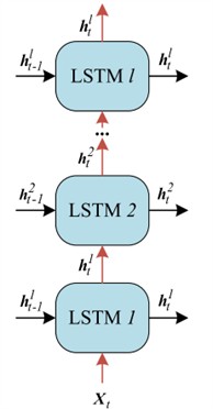
While stacking multiple layers can improve accuracy to a certain extent, it may also lead to degradation issues. This is distinct from the problem of vanishing or exploding gradients, making it difficult for the architecture to stabilize and potentially resulting in an increase in training errors. Empirically, when the number of layers surpasses three, the benefits of stacking begin to diminish, often failing to yield further improvements in performance. Inspired by literature [27], as shown in Fig. 7, This paper presents the concept of residuals, which involves creating shortcuts between the model’s input and output. These shortcuts facilitate the flow of gradient information during backpropagation, effectively conveying the gradient to earlier layers. This mechanism ensures the trainability of deep networks. The formula for stacking with $L$ layers is presented as follows:

19

$C_t^l,h_t^l=LST{M}_{\text{encoder}}^l\left(C_{t-1}^l,h_{t-1}^l,x_t^l\right),\left(1\le t\le T\right),$

20

$x_t^l=\left\{\begin{array}{ll}{h}_t^{l-1}+h_t^{l-2},& \left(3\le l\le L\right),\\ h_t^{l-1},& \left(l=2\right),\\ X_t,& \left(l=1\right).\end{array}\right.$

2.3.2. Decoder

Initially, the LSTM processes the context vector provided by the compressor and sequentially outputs hidden states. Subsequently, a multi-level attention mechanism calculates the weights of these hidden states obtained from the compressor at each time step, resulting in an attention vector $V$. Finally, the neural layer produces the predicted values as concatenated features through a linear transformation.

As shown in Fig. 8, the multi-level attention mechanism outlined in this article consists of two focal systems: one is the temporal focus system (time-focus), and the other is the semantic focus system (meaning-focus).

Fig. 8Multi-level attention mechanism

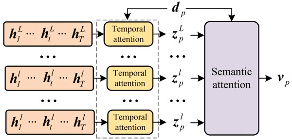
The time-focus system is capable of dynamically selecting the relevant hidden states from each layer of the LSTM for the calculation of time-focus vectors, thereby overcoming the information loss due to feature compression during encoding. Meanwhile, the meaning-focus system evaluates the importance of the information from each LSTM layer for prediction.

2.4. Forecasting framework

The comprehensive prediction framework initially employs the optimized group statistical phase separation technique (EEMD) to decompose the converter variable parameter series into several sub-series, as illustrated in Fig. 9. An adaptive clustering algorithm is subsequently utilized to cluster and reconstruct these sub-series, aiming to reduce the complexity and time consumption of parameter prediction. Following this, multi-level sub-series, along with other equipment parameter sequences, are integrated as multidimensional inputs for a multi-cascade network designed for subsequence prediction. Ultimately, the predicted values from each subsequence are aggregated to derive the final prediction for the target parameter sequence.

Fig. 9Converter parameter prediction framework

2.5. Early warning blur

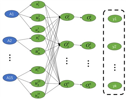
We seek to derive potential early warning information for current converter transformers by analyzing predicted data alongside established expert rules. The early warning information is categorized into distinct classes, with the output of the early warning system being a display of the membership degree of the current data to each of these categories. Therefore, this article selects a fuzzy neural network based on the standard fuzzy model to integrate expert rules, early warning classification and other functions [28]. The fuzzy neural network structure based on the standard fuzzy model is shown in the Fig. 10.

For the input of concurrent parameters, can effectively handle early warning “thresholds” with fuzzy boundaries, uncertainty or imprecision. Within the network, fuzzy set theory is used to describe the fuzzy membership of input variables [29], allowing the network to accept and understand fuzzy inputs and make early warning decisions accordingly.

Fig. 10Fuzzy network

3. Experiment

This article selects 13 state parameters such as winding temperature, dissolved gas in oil, core and clamp grounding current, as shown in Table 3.

Among them, the UHF method is used to detect the partial discharge signal of the converter transformer in the high-voltage laboratory, and the partial discharge detector, UHF sensor and oscilloscope are used to build an experimental platform to obtain experimental data. The partial discharge measurement is carried out in the transformer tank within the lab. The test setup and connections are illustrated in the Fig. 11.

The device includes a high-voltage test power supply with no partial discharge and is specified at 150 kV/AC; and a converter with model number SZ9–2000/35 with a nominal capacity of 2000 kVA and a voltage configuration of 35000±3×2.5 %/10500 V.

Fig. 11Experimental platform

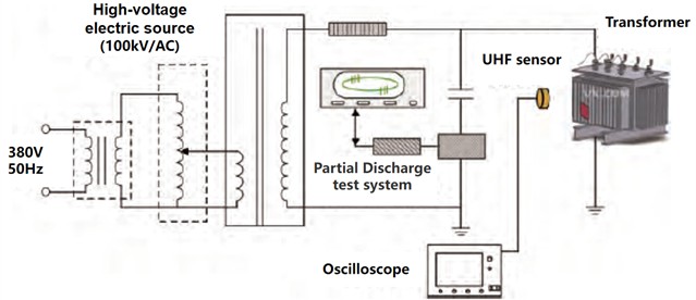
In addition, an electronic PD measuring instrument is included, which integrates components such as a PD sensor, connection capacitors, sense resistors, and calibrators (50pC, 100pC). This sensor is a broadband sensor that follows IEC60270 partial discharge measurement standards.

It is used to detect and calibrate partial discharge levels when evaluating system performance, sensitivity, etc. For data acquisition and analysis, a Lecroy fast oscilloscope system (bandwidth: 2 GHz, sampling rate: 20 GHz) was used in this study. In order to further improve the generalization ability of the prediction model, four standard partial discharge modes are independently designed and placed in the converter cavity, including needle tip corona discharge, suspended metal discharge, air gap discharge between oil-paper insulation layers, and oil-paper surface discharge.

By collecting partial discharge signals from different defects, potential generalization features can be introduced into the subsequent prediction process. For this reason, a defect located at the opening of the converter handle was specially set up in this experiment, so that the defective discharge part was completely immersed in the isolation solution of the converter. This setup not only helps to simulate complex environmental conditions in actual operation, but also captures the real performance of various partial discharge phenomena more accurately, thus providing a more reliable basis for the maintenance of power equipment.

(1) Pin apex glow flaw: 20 mm tall aluminum pin apex probe design, one side of the design is firmly attached to the high-tension side of the converter A-phase sleeve, and the opposite side is hanging in the isolating liquid and does not touch the metal casing wall of the converter, as displayed in Fig. 12(a) depicted.

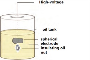
(2) Hanging metal flaws: The spherical probe is fully submerged in isolating liquid, and is reliably linked to the high-tension end of the A-phase bushing of the transformer. Nuts of different sizes are hoisted on the spherical electrode using cable ties, and the electrodes and nuts are blocked by insulating paper. Touch, nut size. The whole flaw is entirely immersed in isolating liquid and is not in contact with the metal casing wall of the converter, as depicted in Fig. 12(b).

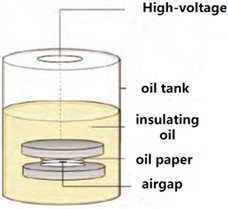
(3) Oil sheet air space flaws: Use three layers of oil paper to superimpose to make the middle of the central layer of. Make apertures of different sizes at the middle of the central layer of oil paper. The size of the oil paper is 5 cm × 5 cm × 5 mm. The gap size is fixed using a partial discharge stress design. One side is firmly linked to the high-tension side of the converter A-phase sleeve, and the opposite side is firmly earthed. The design does not make contact with the metallic surface of the converter, as depicted in Fig. 12(c).

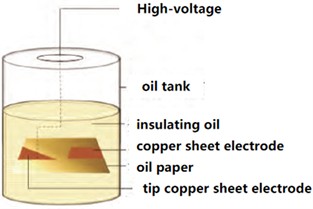
(4) Defects along the surface of the oil paper: Use a tip copper sheet electrode to fix it at one face of the isolating sheet and firmly connect it to the high-tension end of the A-terminal bushing of the transformer. Fix another copper sheet electrode not far away from the oil paper. The size of the oil paper is 12 cm × 12 cm × 5 mm, use copper-clad paper to fix the copper sheet and the insulating oil paper to make the fit closer. The electrical resistance of the isolating cardboard used is >35 kV/mm. Before use, they have been warmed and evacuated to filter out contaminants like humidity, air, fiber fragments, etc., and the processed models are soaked in test converter fluid for > 36 hours prior to the test. During the pressurization test, the whole flaw was completely immersed in isolating liquid and not touching the metallic cabinet wall of the transformer. As depicted in Fig. 12(d).

Fig. 12Transformer typical defect model

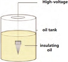
a) Corona discharge model

b) Suspending discharge model

c) Airgap discharge model

d) Surface discharge model

This article uses the stochastic gradient descent algorithm (SGD) and the Ada improvement method to develop the multi-cascade forecast design of this system. Because the suggested forecast design is smooth and differentiable, this may be taught through the conventional backpropagation method. This article uses MSE as the objective function:

where $n$ is the count of forecasted values. and are the $i$-th actual measured value and predicted amount individually. This article chooses RMSE and MAE to assess the effectiveness of the forecast design. The definition is as follows:

For the selected power equipment parameters, all sampling results with interception time in the range from July 2023 to October 2023 constitute a time series as input samples. This time series is collected by sensors distributed on site in a 5-minute cycle, with a total of 12,113 records.

In order to better use data for training and prediction, combine the characteristics of machine learning algorithms and improve the accuracy and training speed of the model, it is necessary to standardize the data and de-standardize the prediction results. We use the Z-Score standardization method to process existing equipment parameter data:

where ${\mu }^{\text{'}}$ and ${\sigma }^{\text{'}}$are the mean and variance of the data respectively.

Moreover, the learning information is split into 80 % learning subset and 20 % verification subset. Next, a sliding frame with an increment of 1 is applied to partition the learning subset into numerous learning instances. Every instance includes T input information units and P information units that require forecasting. For the verification subset, a sliding frame with increment P is utilized to partition the verification subset into numerous verification instances to prevent overlap of forecasted information units. Ultimately, after the design has completed learning on the learning information, the evaluation information is utilized to assess the design’s forecasts. In this research, we modified P and T based on the respective experimental configurations. All trials in this research were executed using the Python coding language (version 3.7). The computer's CPU was Intel I78700K, the GPU was GeForceRTX2080, and the operating system was Microsoft Windows 10. Data processing used the “NumPy” and “PyEEMD” libraries.

We compared it with other 4 methods through short-term and extended forecast experiments. Within this test, the forecast stage sizes $P$ are set to 3, 6, and 9 respectively, and the related input information duration $T$ is also set. Furthermore, considering the time consumption, just 720 information units were forecasted. The compared models are as follows: ARIMAX, SVR, RNN, CNN-LSTM. The parameters $p$, $d$, and $q$ of ARIMAX are automatically adjusted according to Bayesian loss. SVR selects a linear operation core, and the loss setting is established to 1e3. The one-dimensional convolution layer of CNN-LSTM is configured to 3 levels, the core dimension is 3, and maximum pooling Size is 2. Table 4 shows the prediction outcomes of fluid heat information.

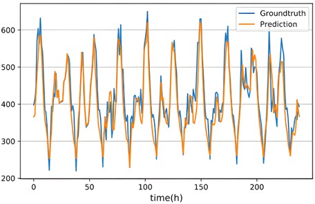
As the prediction step size increases, it is evident that the forecast discrepancy of each technique expands; however, the proposed method consistently outperforms other techniques across both metrics with the smallest increase in discrepancy. Figs. 13-14 illustrates the prediction outcomes of a multi-cascade network, where true values are represented by the cyan line and forecasted values by the amber line.

Fig. 13Oil temperature prediction results

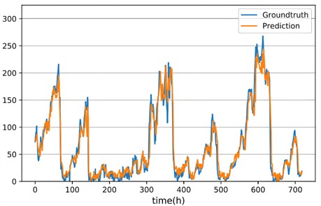
Fig. 14Prediction results of H2 concentration in oil

Based on the system log, inspection report, the stated UHF partial discharge experimental platform, and the GB/T17468-2019 transformer standard, fault categories have been classified into abnormal partial discharge, abnormal winding temperature, abnormal clamp core current, abnormal main body oil level, and abnormal oil chromatography. The corresponding converter transformer equipment parameters include winding temperature, core grounding current, clamp grounding current, oil temperature, oil pressure, dissolved gases in oil, along with 13 other equipment parameters [30] as shown in Table 5.

In order to obtain the fault data used, 74 % of the actual operating data in a real UHV converter station in China from January 2023 to June 2023 was found to be stable and normal. It is not easy to obtain a large amount of equipment abnormal data for experiments. Therefore, a total of 1,200 pieces of actual operating sampling data of abnormal data were used as the basis. According to the “Transformer Abnormality Guidelines”, platforms such as the above-mentioned UHF partial discharge experiment were artificially introduced to simulate different faults for experiments. The training process is as follows:

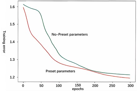
Two strategies are used in the training process: one is to preset network parameters based on expert experience, and the other is to not preset any network parameters. Although both paths achieve similar training results, it is observed that the model with parameter presets exhibits greater efficiency in the training phase and reaches lower training error levels faster as shown in Fig. 15. It also shows that by presetting network parameters, the knowledge contained in expert rules can be effectively embedded into the model structure, so that the fuzzy neural network carries certain prior knowledge before the training is officially started.

Fig. 15Whether to set the training error of the weight

The parameters corresponding to the fuzzy neural network model were sampled, and a total of 2450 prediction anomaly samples of the multi-cascade network were obtained. The classification results are as Table 6. It can be seen that the predicted data can be used to infer the early warning categories to achieve multi-type accuracy. As shown in Table 6, all remain above 90 %.

4. Conclusion

This article mainly focuses on the research on the status early warning of UHV converter transformers, aiming to solve the problem of inaccurate prediction of non-stationary parameters of equipment and improve the diversity and flexibility of early warning results. By designing a commutation change state early warning system that combines DPR-KLdiv-EEMD decomposition and clustering, multi-cascade network and fuzzy set ideas, it effectively copes with the problem of non-stationary parameter prediction of equipment and improves the diversity and flexibility of early warning results. It has good prediction performance and robustness in experimental verification. In the future, more attention will be paid to the network replacement of LSTM and the optimization direction of multi-cascade architecture, so as to make the early warning parameters more diversified.