Stodola-Vianello iteration method for the free flexural vibration frequencies of Shimpi’s single variable shear deformable beams

1. Introduction

Beams are structural members that are extensively used in aerospace, mechanical, civil and automobile engineering. They are known to have longitudinal dimensions that are much larger than the cross-sectional dimensions. They carry transverse loadings by the development of flexural deformations. They can be subjected to static, dynamic and/or in-plane loads and hence can develop flexural responses. The focus of this paper is on dynamic response of beams.

Beams that are subjected to time varying forces are prone to resonance failures when the inherent natural frequencies of the beam are equal to the frequencies of external excitation due to the applied load. The natural frequencies of structures and beams have been found to depend upon their stiffness and intertial properties.

In order to avoid resonant failures of beams, it is a vital step to conduct natural frequency analysis in order to determine the resonant frequencies at which failures would occur upon coincidence with the dynamic loading frequencies.

The dynamic behaviour of beam is dependent on the geometry of the beam among other factors. When the ratio of depth of the cross-section to the span $l$ of the beam is less than or equal to 0.05, the beam is called a thin or slender beam. When the ratio of depth to span is greater than 0.05, the beam becomes moderately thick or thick. Beams are thus classified as thin when $h/l\le \text{0.05}$, thick if $h/l>\text{0.05}$.

Several theories have been developed for beam vibration analysis. The Euler-Bernoulli beam theory (EBBT) is the classical beam theory (CBT) which has been found suitable for thin beams. The theory has been formulated for static flexural, dynamic and buckling problems [1-5]. The EBBT was derived using the Euler-Bernoulli-Navier hypothesis that vertical lines on the plane cross-sections that are initially normal to the longitudinal neutral axis before deformation would remain plane and normal to the longitudinal neutral axis after deformation due to the applied loads [2], [4]. This Navier-Euler-Bernoulli orthogonality hypothesis implies that there are no transverse shear deformations. Shear strains which can produce non-planar cross-sectional deformations are ignored in the EBBT [6].

The formulation of EBBT equations thus discountenance transverse shear deformations rendering the theory unsuitable for moderately thick and thick beams where transverse shear deformation effect could significantly affect the vibration characteristics.

Erdelyi and Hashemi [7] used the EBBT for deriving dynamic stiffness matrix (DSM) to relate sinusoidally varying loads to sinusoidally varying displacements at the beam ends for delaminated multilayered beams. Their DSM was then used to study the natural frequencies and mode shape of two-layer beam systems.

In order to provide other beam theories to incorporate shear deformation effects, Timoshenko [8] derived the first order shear deformation beam theory called the Timoshenko beam theory (TBT) which has been extended by several scholars to describe vibration and buckling beam behaviours.

TBT considers the deformations to be made of the sum of bending and shear deformations and thus is applicable to moderately thick beams. However, the TBT yields constant transverse shear strain distribution across the beam depth, thus resulting in a non-zero shear stress at the beam’s top and bottom surfaces in violation of the transverse shear stress-free boundary conditions at the beam’s top and bottom surfaces (Ike, [2]) shear modification factors which are problem dependent and dependent on cross-sectional shape were introduced in order to ensure that the accurate strain energy of deformation is obtained in the theory.

Cowper [9] researched on the improvements of the TBT and developed analytical expressions for the shear stress modification factors in terms of the cross-section geometry and Poisson’s ratio. Mindlin improved the TBT by simplifying the transverse shear strain as a constant distribution through the beam depth profile [6]. Mindlin used a shear coefficient, $k_s$, to properly represent the strain energy of the beam and to include the effect of non-constant shear stresses and strains. Values of $k_s$ for different cross-sectional shapes were presented by Cowper [9].

Several researches were inspired by the need to solve the issues associated with the EBBT, TBT and their improvements. These researches led to the development of shear deformation theories (SDTs), higher order shear deformation theories (HoSDTs) and refined beam theories (RBTs).

SDTs, HoSDTs and RBTs were all developed by several investigators with the principal concern to satisfy the transverse shear stress free conditions at the top and bottom beam surfaces $(z=\pm h/2)$ while also incorporating the transverse shear deformation into the formulation. Shear shape functions were used in various formulations of SDTs, HoSDTs and RBTs in order to ensure that the shear stress free boundary conditions are satisfied. These shear shape functions used are derived such that the shear stress free boundary conditions are satisfied. The commonly used functions are: polynomials, trigonometric, hyperbolic and exponential functions.

Apart from propositions on the several shear shape functions researchers have constructed refined beam theories that seek to reduce the number of unknown displacement and/or stress terms in beam theories. Touratier [10] presented exact solutions to the thick beam vibration problem.

Shear deformable beam theories have been studied by Pakhare et al. [11]; Shimpi et al. [12]; Vascocelos et al. [13], Levinson, [14]; Murty [15] and Shi and Voyiadjis [16]. Levinson [14] presented a third order shear deformable rectangular beam theory for bending analysis but did not consider vibration behaviour. Murty [15] derived a shear deformation theory for the dynamic analysis of beams and used it to develop natural frequencies of vibrating beams under simple supports. Shi and Voyiadjis [16] derived a sixth-order theory of shear deformable beams using the methods of variational calculus. Stephen and Levinson [17] derived a shear deformable theory to incorporate shear strain effects.

Ghugal and Sharma [18] developed a shear deformable beam theory for bending and vibration analysis using hyperbolic shear function to ensure the satisfaction of the transverse shear stress-free boundary conditions. Pakhare et al. [11] used the methods of variational calculus to develop variationally consistent and inconsistent equations for the natural transverse vibration characteristics of shear deformable beams made of homogeneous isotropic linear elastic materials. They used Fourier series method to obtain accurate eigensolutions for the natural frequencies.

Shimpi et al. [12] developed shear deformation beam theory using a single displacement variable as the unknown in their displacement based formulation. Thai et al. [19] presented a deformation theory for non-local beams.

Higher order shear deformable beam theories have been investigated by Razouki et al. [20], Zioù et al. [21] and Heyliger and Reddy [22]. Heyliger and Reddy [22] developed finite element stiffness and inertial matrices based on a higher order shear deformation beam theory for the bending and vibration problems. Zioù et al. [21] used a higher order shear deformable theory for the static bending analysis of functionally graded (FG) beams, but did not extend their work to vibration analysis.

Razouki et al. [20] also used the differential transform method (DTM) to solve bending problems of thick FG beams formulated using HoSDT, but they did not consider vibration problems. Ghugal and Shimpi [23] presented a concise review of refined shear deformation theories for isotropic and anisotropic laminated beams. Sayyad and Ghugal [24] developed single variable refined beam theories for the bending, buckling and natural vibration analysis of homogeneous beams.

Ibearugbulem et al. [25] used the principle of energy minimization to determine the natural vibrating frequencies of refined beams. Shimpi et al. [26] developed simple two variable refined beam theory for isotropic, homogeneous, rectangular beams, but did not consider vibration cases. Sayyad [27] presented a comparison of different RBTs for the bending and natural vibration behaviour of thick beams.

This study adopts the Stodola-Vianello vibration method for solving the resulting thick beam vibrating problem. The Stodola-Vianello iteration method has been sparsely used.

Dong et al. [28] presented applications of the Stodolla-Vianello and Gram-Schmidt schemes for solving eigen problems of frequencies and mode shapes. They found reduction in computational effort and computer memory space as advantages of the iterative method.

Chennit et al. [29] used the Stodola-Vianello iteration method to determine the periods and mode shapes for uniform shear wall buildings, which are important dynamic characteristics essential for the analysis of seismic response of multi-storey buildings. Their research provided new database of vibration modes of multi-storey buildings with reinforced concrete (RC) shear walls.

Ike [30], [31] used the Stodola-Vianello iteration method to obtain exact buckling load solutions for simply supported Euler-Bernoulli beam on Winkler and Pasternak foundations respectively. Sinusoidal buckling shape functions were used in the derived Stodolla-Vianello iteration equations to obtain the next eigenfunction and the convergence rule at the ($n+1$)th iteration was used to find the eigenvalues which were used to obtain the exact buckling loads at any $n$th buckling mode. Ofondu et al. [32] applied the SVIM for the critical buckling load determination of Euler columns.

In another study Ike [33] used the Stodola-Vianello iteration method to determine approximate buckling load solutions using polynomial buckling shape functions in the Stodola-Vianello iteration formula for simply supported thin beam on Winkler foundation. Ike et al. [34], [35] have also applied the Stodolla-Vianello iteration method to obtain sufficiently accurate approximate buckling solutions for clamped-clamped thin beam on Winkler and Pasternak foundations respectively. In a recent work Ike [36] used the SVIM for the critical buckling load solutions of Euler-Bernoulli beams on two-parameter foundations using polynomial basis functions.

A review of literature reveals that very few studies have been done on the subject of transverse vibrations of thick beams modelled using shear deformable theories; and the Stodola-Vianello method has never been used for solving the governing differential equations of vibration. The aim of this paper is to derive from first principles Shimpi’s single variable shear deformation theory for transverse flexural vibrations for free and forced vibration, and then apply Stodolla-Vianello iteration method for the first time, to solve the resulting governing equation of motion for simply supported boundary conditions and natural harmonic vibrations.

2. Novelty of the study

The novelty of the study are:

– The first principles systematic presentation of the derivation of the governing equation of motion using the method of differential equation of dynamic equilibrium of an infinitesimal beam element and consideration of strain-displacement equation, stress-strain equations of linear elasticity and Shimpi et al. [12] assumptions of the displacement field components.

– The Stodola-Vianello iteration method is applied for the first time in a systematic way to formulate the Stodola-Vianello iteration equations and to obtain convergent solutions for simply supported boundary conditions.

3. Results

$F_n\left(x\right)$ for the $n$th vibration mode which satisfies the simply supported boundary conditions is:

Since:

where ${\stackrel{-}{F}}_n$ is the amplitude of $F_n\left(x\right)$ for the $n$th vibration mode:

Applying the boundary conditions:

Hence:

At convergence:

So:

Division by $\stackrel{-}{F}\mathrm{s}\mathrm{i}\mathrm{n}\frac{n\pi x}{l}$ gives:

Rearranging the equation gives:

Further re-arrangement gives:

Lets define the dimensionless frequency parameter ${\theta }_n$ as:

Then the characteristic equation is expressed in terms of ${\theta }_n$ as:

But for rectangular cross-sections:

So:

This can be considered a quadratic equation in ${\theta }_n^2$ and the roots of the equation can be found using the quadratic formula. Using ${\theta }_n^2$, ${\omega }_n^2$ can be found as:

So:

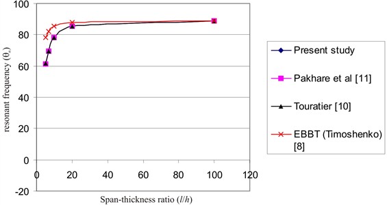
The results for ${\theta }_n$ are presented in terms of various values of $l/h$ and for $\mu =\text{0.30}$ in Tables 1, 2, 3 and 4. The variations of ${\theta }_n$ with $l/h$ are also presented for the first three mode of vibration in Figs. 1, 2, and 3.

4. Discussion

In this paper, Shimpi’s single variable shear deformation beam theory for forced and free transverse flexural vibrations have been derived from first principles and then the Stodola-Vianello iteration method applied for the first time, in a novel systematic way to solve the resulting governing equation of motion for simply supported boundary conditions and natural harmonic vibrations. The derivation was based on the differential equation of dynamic equilibrium method, rather than the commonly found variational calculus procedure. Differential equations of dynamic equilibrium, stress-strain relations and the strain displacement relations of small displacement linear elasticity were simultaneously applied with the Shimpi et al. [12] expressions for the assumed displacement field in order to determine the partial differential equations of motion. The obtained boundary value problem (BVP) which is a non-homogeneous PDE for force vibration, simplifies to a homogeneous PDE for free vibrations due to the absence of the excitation forcing force in the case of free (natural) vibration. The study focused on free vibration, and hence entailed the solution of the homogeneous PDE using Stodola-Vianello iterative method. For the simply supported thick beam vibration problem, the BVP is represented by Eq. (38b) and the boundary conditions Eqs. (39a) and (39b). For harmonic vibrations and expected harmonic response the PDE simplifies to a fourth order ordinary differential equation (ODE) as the modal equation given by Eq. (48). This fourth order modal equation is expressed using SVIM as the system of iterative equations – Eqs. (51b) and (54).

The use of sinusoidal eigenfunctions at the $n$th vibration mode which is the exact eigenfunction for a simply supported beam in the Stodola-Vianello iteration equation led to the determination of the four constants of integration. The application of the convergence rule at the $n$th vibration mode as expressed by Eq. (61) resulted in the algebraic eigenvalue problem given by Eq. (63). Further rearrangements of Eq. (63) and simplification for beams of rectangular cross-sections gave the fourth degree characteristic eigenvalue equation in terms of ${\theta }_n$ as Eq. (71). Hence ${\omega }_n$ is found expressed in terms of ${\theta }_n$ as Eq. (72c). The results for ${\theta }_n$ are presented in terms of various values of $l/h$ for $\mu =\text{0.30}$ in Tables 1, 2, 3 and 4 and in Figs. 1, 2, and 3.

Tables 1-4 and Figs. 1-3 also compare the obtained values of ${\theta }_n$ for various vibration modes $n=$ 1, $n=$ 2, $n=$ 3 and $n=$ 4 with previous values presented by Shimpi et al. [26], Touratier [10], Timoshenko [8] and Pakhare et al. [11].

Table 1 shows that the present study is identical with previous studies by Shimpi et al. [26] and Pakhare et al. [11] who both used Navier’s series method to solve the single variable shear deformable beam problem. Table 1 also illustrates that the present SVIM results are identical with the Navier solutions of the flexural vibration results of thick beams modelled using two-variable shear deformable beam theory as presented by Pakhare et al. [11] and Shimpi et al. [26]. Table 1 further compares the SVIM present results with exact results presented by Touratier [10] and shows that for $l/h$ equal to 10, 20, and 100, the present SVIM results are identical with exact results by Touratier [10], but –0.01 % different from the exact results for $l/h$ equal to 5 and 20/3. The Table 1 further illustrates that the EBBT results differ from the exact results of Touratier [10] by 0.01 % for $l/h$equal to 100; 0.32 % for $l/h$ equal to 20 and the errors increase to 4.70 % for $l/h$ equal to 5.0.

Fig. 1Graph of θn vs l/h for n= 1 (simply supported thick beams)

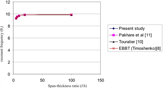
Fig. 2Graph of θn vs l/h for n= 2 (simply supported thick beams)

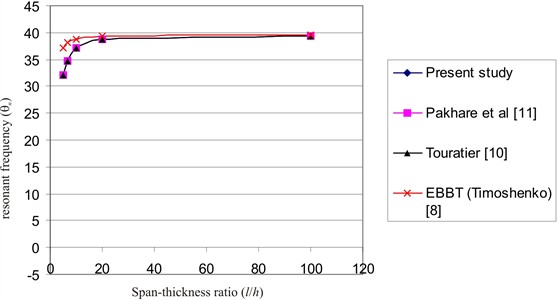
Fig. 3Graph of θn vs l/h for n= 3 (simply supported thick beams)

Similar observations are noted for Table 2 which shows the natural frequency results for the second mode of flexural vibration for the thick beam problem. Table 2 shows that the SVIM results for ${\theta }_n$ are identical with the SVSDBT results obtained using Navier’s method by Pakhare et al. [11] and Shimpi et al. [26] and in close agreement with TVSDBT solutions using Navier method by Pakhare et al. [11] and Shimpi et al. [26]. Comparison of present results with Touratier [10] exact solution shows a negligible difference of 0 % for $l/h=$ 100, 0 % for $l/h=$ 20, –0.01 % for $l/h=$ 10, –0.04 % for $l/h=$ 20/3 and –0.09 % for $l/h=$5. The EBBT results of Timoshenko [8] presented in Table 2 show the unsuitability of the EBBT method for eigensolution of the problem especially for $l/h$ < 10 due to solution errors exceeding 4.70 %.

Table 3 shows values of ${\theta }_n$ for $n=$ 3 for the flexural vibration problem of the thick SVSDBT studied using SVIM. Table 3 shows that the SVIM results are identical with Navier results presented by Shimpi et al. [26] and Pakhare et al. [11] using SVSDBT, and closely agree with Navier method results presented by Shimpi et al. [26] and Pakhare et al. [11] using TVSDBT. The present SVIM results show negligible differences of 0 % for $l/h=$ 100, –0.01 % for $l/h=$ 20, –0.04 % for $l/h=$ 10, –0.12 % for $l/h=$ 20/3 and –0.26 % for $l/h=$5 from the Touratier [10] exact results. The EBBT results as presented by Timoshenko [8] and shown in Table 3 is unsuitable for the eigenfrequency solution because of the solution error of more than 9.63 % for $l/h=$ 10; and greater error for $l/h$ < 10.

Table 4 shows values of ${\theta }_n$ for $n=\text{4}$ for the flexural vibration of the thick SVSDBT studied using SVIM. Table 4 illustrates that the SVIM result for ${\theta }_n$ for $n=$ 4 are identical with Navier results presented by Shimpi et al. [26] and Pakhare et al. [11] for thick SVSDBT beams, and closely agree with Navier method results presented by Shimpi et al. [26] and Pakhare et al. [11] for thick TVSDBT beams. The Table 4 further illustrate that the present SVIM results show insignificant differences of 0 % for $l/h=$ 100; –0.01 % for $l/h=$ 20; –0.09 % for $l/h=$ 10, –0.26 % for $l/h=$ 20/3 and –0.56 % for $l/h=$ 5 from the Touratier [10] exact results. Table 4 also illustrate the unsuitability of the EBBT results presented by Timoshenko [8] for the eigen solution because of the unacceptable errors of 4.70 % for $l/h$ < 20 associated with the EBBT theory applied to the flexural vibration problems of thick beams for the fourth mode of vibration.